Quarto

Club Bioinfo, Jouy

Mahendra Mariadassou

MaIAGE

Cédric Midoux

PROSE & MaIAGE

April 13, 2023

Notebooks

RMarkdown & Jupyter Notebook

• Framework for data science
• Easiest way to make computational documents
  • An (optional) YAML header surrounded by ---
  • R/Python code chunks surrounded by ```
  • Text mixed with simple text formatting with markdown.
• Export knit and processed by pandoc to produce a complete report containing all text, code and results.

Analyze. Share. Reproduce.

RMarkdown & Jupyter Notebook

R Markdown: The Definitive Guide

R Markdown Cookbook

IPython Cookbook

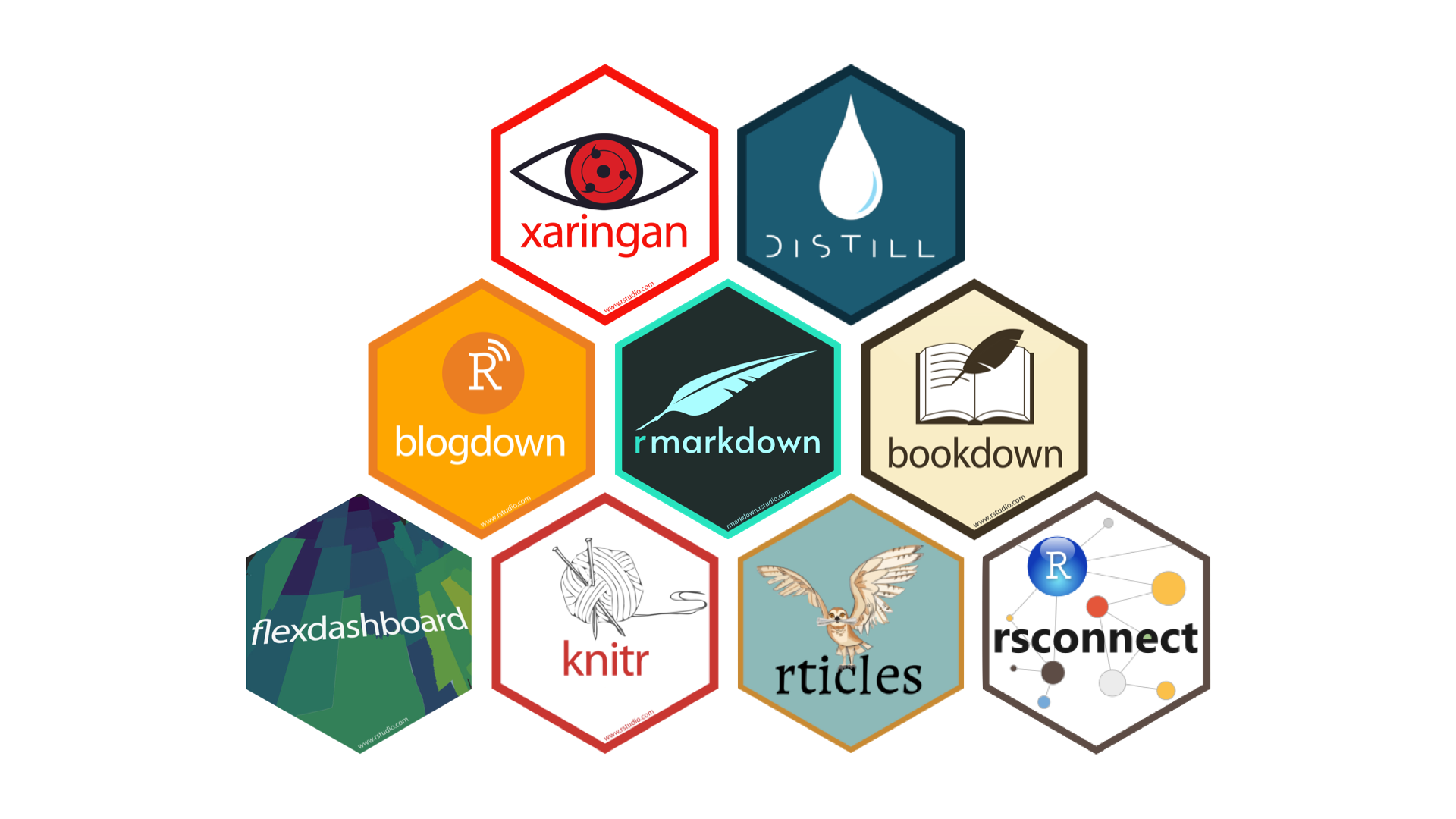
The R Markdown ecosystem

Quarto: Next generation R Markdown

Quarto unifies and extends the R Markdown ecosystem

Quarto is a new, open-source, scientific and technical publishing system

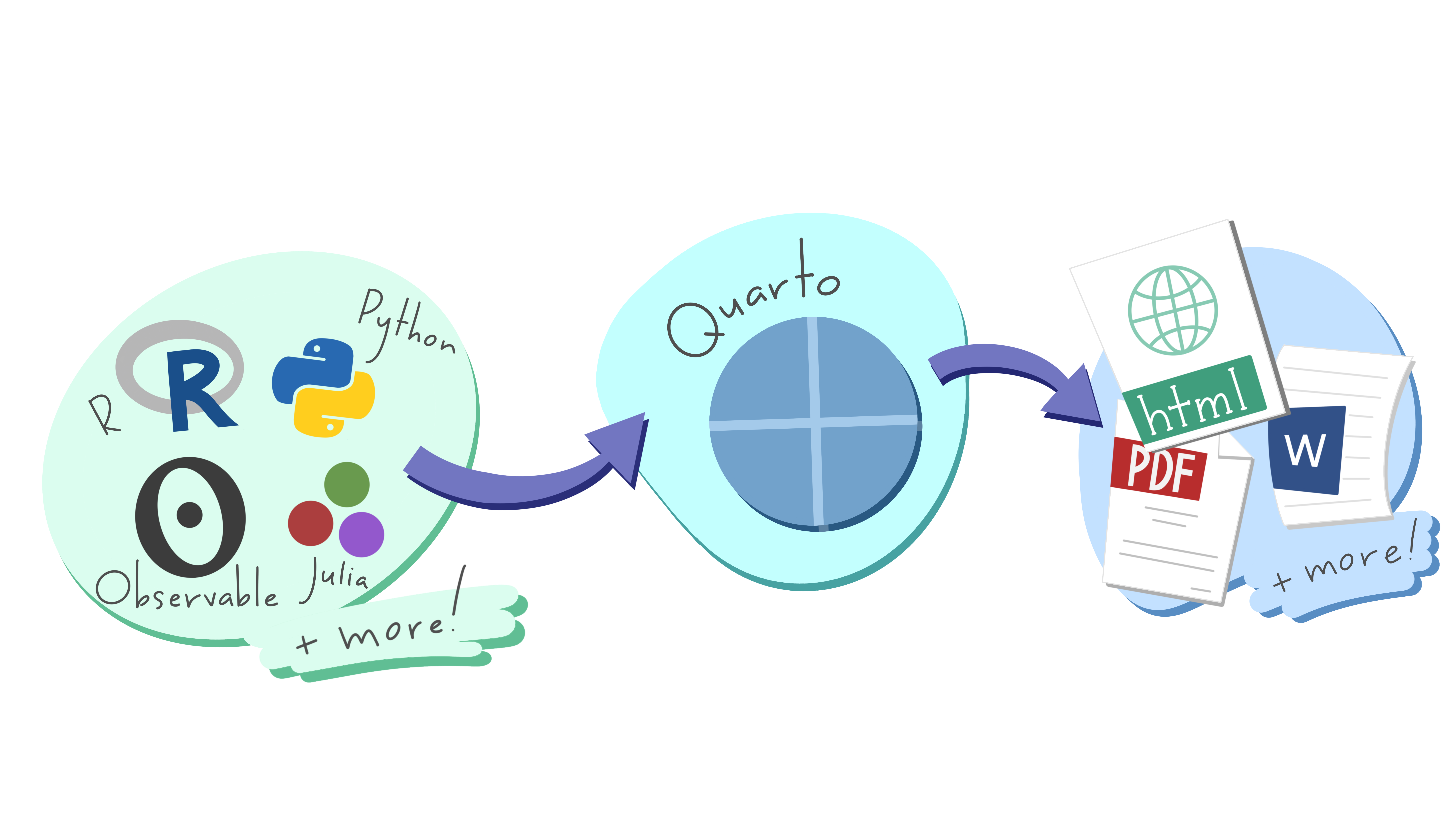
So what is Quarto ?

Quarto is a command line interface (CLI) that renders plain text formats (.qmd, .rmd, .md) OR mixed formats (.ipynb/Jupyter notebook) into static PDF/Word/HTML reports, books, websites, presentations and more

More than just knitr

Quarto powers Computo

A journal of the French Statistical Society SFdS - ISSN 2824-7795

Benefits of Quarto

From the R user point of view: Decoupling from R

• Quarto is multi-core and multi-engine
• Dedicated CLI
• Unlike Rmd / Jupyter notebooks, Quarto is not tied to a language¹
• Compatible with your editor (Jupyter Lab, Neovim, VS Code, RStudio, etc), with many visual edition modes available
• Makes collaboration easier

1. You can use Python in Rmd within Rstudio and R in Jupyter notebooks but few people do.

Quarto highlights

• Consistent implementation of attractive and handy features across outputs: tabsets, code-folding, syntax highlighting, etc.
• More accessible defaults as well as better support for accessibility.
• Guardrails, particularly helpful for new learners: YAML completion, informative syntax errors, etc.
• Support for other languages like Python, Julia, Observable, and more via Jupyter engine for executable code chunks.

Native support (I)

• citations: bibliography files (bibtex), bibliography style (csl)

---
title: "My Document"
bibliography: references.bib
csl: nature.csl
---

"On est super à la bourre!" [@Mariadassou2023,@Midoux2023]

• cross-references for figures (fig-), tables (tbl-), sections (sec-), equations (eq-), (thm-), etc

## Introduction {#sec-introduction}

See @sec-introduction for additional context.

Native support (II)

• Appendices
  • automatic: references, footnote and (self-)citation
  • manual: acknowledgements, technical proofs, etc

## Acknowledgments {.appendix}

We are grateful to all people who made beautiful slides 
which greatly inspired us. 

• Document License (as Reuse section)

---
license: "CC BY"
---

Extensions

• include-code-files : code from source files
• fontawesome, academicons, … : Use icons
• collapse-social-embeds : include social items.
• Journal Articles Template
• quarto-inrae-extension : INRAE formats for HTML, PDF, Docx, Revealjs, and Beamer, thanks to @david_carayon
• …

Quarto Extensions

Outputs

Quarto CLI orchestrates each step of rendering

Quarto makes moving between formats straightforward

Document HTML

lesson-1.qmd

title: "Lesson 1"
format: html

Document PDF

lesson-1.qmd

title: "Lesson 1"
format: pdf

Presentation

lesson-1.qmd

title: "Lesson 1"
format: revealjs

Book

_quarto.yml

project:
  type: book
  output-dir: _book

Website

_quarto.yml

project:
  type: website
website: 
  navbar: 
    left:
      - lesson-1.qmd

And more in the Gallery …

Continuous Deployment

GitLab Pages

• The app’s built output files are in a folder named public

• _quarto.yml

project:
  type: website
  output-dir: public

• .gitlab-ci.yml

# The Docker image that will be used to build your app
image: rocker/verse:4.2

# Functions that should be executed before the build script is run
before_script:
  - quarto install extension davidcarayon/quarto-inrae-extension --no-prompt

pages:
  script:
    - quarto render
  artifacts:
    paths:
      # The folder that contains the files to be exposed at the Page URL
      - public
  rules:
    # This ensures that only pushes to the default branch will trigger
    # a pages deploy
    - if: $CI_COMMIT_REF_NAME == $CI_DEFAULT_BRANCH

Github Actions for Quarto

1. quarto-dev/quarto-actions/setup - Install Quarto
2. quarto-dev/quarto-actions/render - Render project
3. quarto-dev/quarto-actions/publish - Publish project

• Doc

Demo: RStudio integration

Demo: presentations

Easy presentations

Toggle the slide menu with the menu button (or press m) to go to other slides and access presentation tools.
Some other tools like PDF Export in this settings.

 

Press Escape (or press o) to toggle overview mode.

Use the chalkboard button (or press b) to toggle the chalkboard.

Use the notes canvas button (or press c) to toggle drawing on top of the current slide.

Lightweight syntax

Callout-blocks

::: {.callout-note}
Five shades of callouts: `note`, `warning`, 
`important`, `tip`, and `caution`.
:::

Note

Five shades of callouts: note, warning, important, tip and caution.

Diagrams

```{mermaid}
flowchart LR
    A{node 1}-- is -->B(node 2)
    A-- has -->C[node 3]
```

flowchart LR
    A{node 1}-- is -->B(node 2)
    A-- has -->C[node 3]

Videos

{{< youtube dM7x1PNZDo0 >}}

Pretty Code

• Over 20 syntax highlighting themes available
• Default theme optimized for accessibility

# Define a server for the Shiny app
function(input, output) {
  
  # Fill in the spot we created for a plot
  output$phonePlot <- renderPlot({
    # Render a barplot
  })
}

Code Animations

• Over 20 syntax highlighting themes available
• Default theme optimized for accessibility

# Define a server for the Shiny app
function(input, output) {
  
  # Fill in the spot we created for a plot
  output$phonePlot <- renderPlot({
    # Render a barplot
    barplot(WorldPhones[,input$region]*1000, 
            main=input$region,
            ylab="Number of Telephones",
            xlab="Year")
  })
}

Code highlighting

• Highlight specific lines for emphasis
• Incrementally highlight additional lines

```{r}
#| code-line-numbers: "|2|9-10"
#| output-location: column
library(ggplot2)
ggplot(
  mtcars, 
  aes(hp, mpg, color = am)
) +
  geom_point() +
  geom_smooth(formula = y ~ x, method = "loess")
```

Widgets

Native support for JupyterWidgets (Jupyter) and htmlwidgets (R/knitr)

```{r}
#| output-location: column-fragment
library(leaflet)
leaflet(width = "480px") %>%
  addTiles() %>%
  addMarkers(
    lat=48.7660, 
    lng=2.1830, 
    popup="We are here!"
  )
```

Transitions (I)

Use . . . to indicate a break at an arbitrary location

Let's have a look at `iris`

. . . 

```{r}
head(iris) |> knitr::kable()
```

Let’s have a look at iris

Sepal.Length	Sepal.Width	Petal.Length	Petal.Width	Species
5.1	3.5	1.4	0.2	setosa
4.9	3.0	1.4	0.2	setosa
4.7	3.2	1.3	0.2	setosa
4.6	3.1	1.5	0.2	setosa
5.0	3.6	1.4	0.2	setosa
5.4	3.9	1.7	0.4	setosa

Fragments

::: {.fragment}
Fade in
:::

::: {.fragment .fade-out}
Fade out
:::

::: {.fragment .strike}
Strike text
:::

::: {.fragment .fade-in-then-out}
Fade in, then out
:::

::: {.fragment .fade-up}
Slide up while fading in
:::

Fade in

Fade out

Strike text

Fade in, then out

Slide up while fading in

Column output

```{r}
#| code-line-numbers: "|3"
#| output-location: column
ggplot(mtcars, aes(hp, mpg)) +
  geom_point() +
  geom_smooth(formula = y ~ x, method = "loess")
```

```{r}
#| code-line-numbers: "|3"
#| output-location: column-fragment
ggplot(mtcars, aes(hp, mpg)) +
  geom_point() +
  geom_smooth(formula = y ~ x, method = "loess")
```

Tabset output

• Code
• Plot
• Under the hood

```{r}
p <- ggplot(mtcars, aes(hp, mpg)) +
  geom_point() +
  geom_smooth(formula = y ~ x, method = "loess")
```

::: {.panel-tabset}

### Plot code

```{r}
#| echo: fenced
p <- ggplot(mtcars, aes(hp, mpg)) +
  geom_point() +
  geom_smooth(formula = y ~ x, method = "loess")
```

### Plot

```{r}
p
```

:::

Easy layouts

• Code
• Plot

• Use negative values for white space

```{r}
#| eval: false
#| fig-subcap:
#|   - "boring 🥱"
#|   - "boooring 🥱🥱"
#|   - "boooriiing 🥱🥱🥱"
#| fig-height: 2
#| layout: [[40,-20,40], [100]]
p
p
p
```

boring 🥱

 

boooring 🥱🥱

boooriiing 🥱🥱🥱

Observable graphs

Turn presentations into applications with Observable and Shiny. Use component layout to position inputs and outputs.

viewof bill_length_min = Inputs.range(
  [32, 50], 
  {value: 35, step: 1, label: "Bill length (min):"}
)
viewof islands = Inputs.checkbox(
  ["Torgersen", "Biscoe", "Dream"], 
  { value: ["Torgersen", "Biscoe"], 
    label: "Islands:"
  }
)

filtered = transpose(data).filter(function(penguin) {
  return bill_length_min < penguin.bill_length_mm &&
         islands.includes(penguin.island);
})

Plot.rectY(filtered, 
  Plot.binX(
    {y: "count"}, 
    {x: "body_mass_g", fill: "species", thresholds: 20}
  ))
  .plot({
    facet: {
      data: filtered,
      x: "sex",
      y: "species",
      marginRight: 80
    },
    marks: [
      Plot.frame(),
    ]
  }
)

Demo: websites

Productions Migale

• Site web (en cours de construction)
• Slides Cédric

RMarkdown vs. Quarto

Should I Switch to Quarto?

Yihui Xie

Should you switch to Quarto? Not necessarily. If you find R Markdown meet your need, you can definitely stay there. It is not imperative to switch. - Yihui Xie

https://yihui.org/en/2022/04/quarto-r-markdown/

Some Killer Apps for Quarto (HTML)

• Standardized YAML across formats
• Decoupled from RStudio
• More consistent presentation across formats
• Tab Panels
• Code Highlighting
• Output Freezing
• Precise Layouts

RMarkdown

```{r setup, include=FALSE}
knitr::opts_chunk$set(echo = TRUE)
library(tidyverse)
library(DT)
library(ggimage)
```

Quarto

```{r}
#| label: "setup"
#| include: false
knitr::opts_chunk$set(echo = TRUE)
library(tidyverse)
library(DT)
library(ggimage)
```

Options are moved to within the code chunk using #| (hash-pipe) for each line

How to move to Quarto

1. Install Quarto
2. Start a Quarto Project
3. Convert your Rmarkdown Documents
   • Change your output: to the corresponding format: in your YAML
   • Use knitr::convert_chunk_header() to convert your code blocks (outputs a .qmd file)
4. Render your files
5. For websites: edit your _quarto.yml file if necessary
6. Publish

Take Home Message

• Quarto is a new, open-source, scientific and technical publishing system
• Quarto supports multiple languages / IDEs
• Quarto standardizes a lot of outputs
• Does a better job of one document, many outputs
• Lots of publishing features (references, figures, etc.)
• Very well documented

Sources

Sources

• Quarto, Get Started
• Guides
• Hello Quarto & Keynote
• Quarto presentations
• Get started with Quarto workshop
• With Quarto Coming, is R Markdown Going Away? No.