Analyse de données NGS sous Galaxy
Module 8 bis
April 23, 2024
Introduction
Practical informations
- 9h00 - 17h00
- 2 breaks morning and afternoon
- Lunch at INRAE restaurant (not mandatory)
- Questions allowed
- Everyone has something to learn from each other
Better know you
Who are you?
- Institution / Laboratory / position
What is your scientific topic?
- Studied ecosystem
- Scientific question
- Experimental design
What is your background?
- What are your needs in NGS data analysis?
- Do you have already dealt with NGS data?
- Have you ever used Galaxy ?
Better know us
- Open infrastructure dedicated to life sciences
- Computing resources, tools, databanks…
- Dissemination of expertise in bioinformatics
- Design and development of applications
- Data analysis
Data analysis service
- We are specialized in genomics/metagenomics
- Bioinformaticians and Statisticians
- More than 110 projects since 2016
- 2 types of services
- Collaboration or Accompaniement
Training objectives
After this training day, you will know:
- the characteristics of the main types of sequencers
- how to do a quality control of the raw sequences
- how to assemble a (small) genome
- how to align reads to a reference genome
- how to explore graphically an alignment
- how to compare assemblies
Program
Morning
- Introduction & Round table
- Sequencing technologies
Break
- Quality Control
- Data cleaning
- Assembly
Afternoon
- Assembly evaluation and comparison
Break
- Mapping
- Visualisation
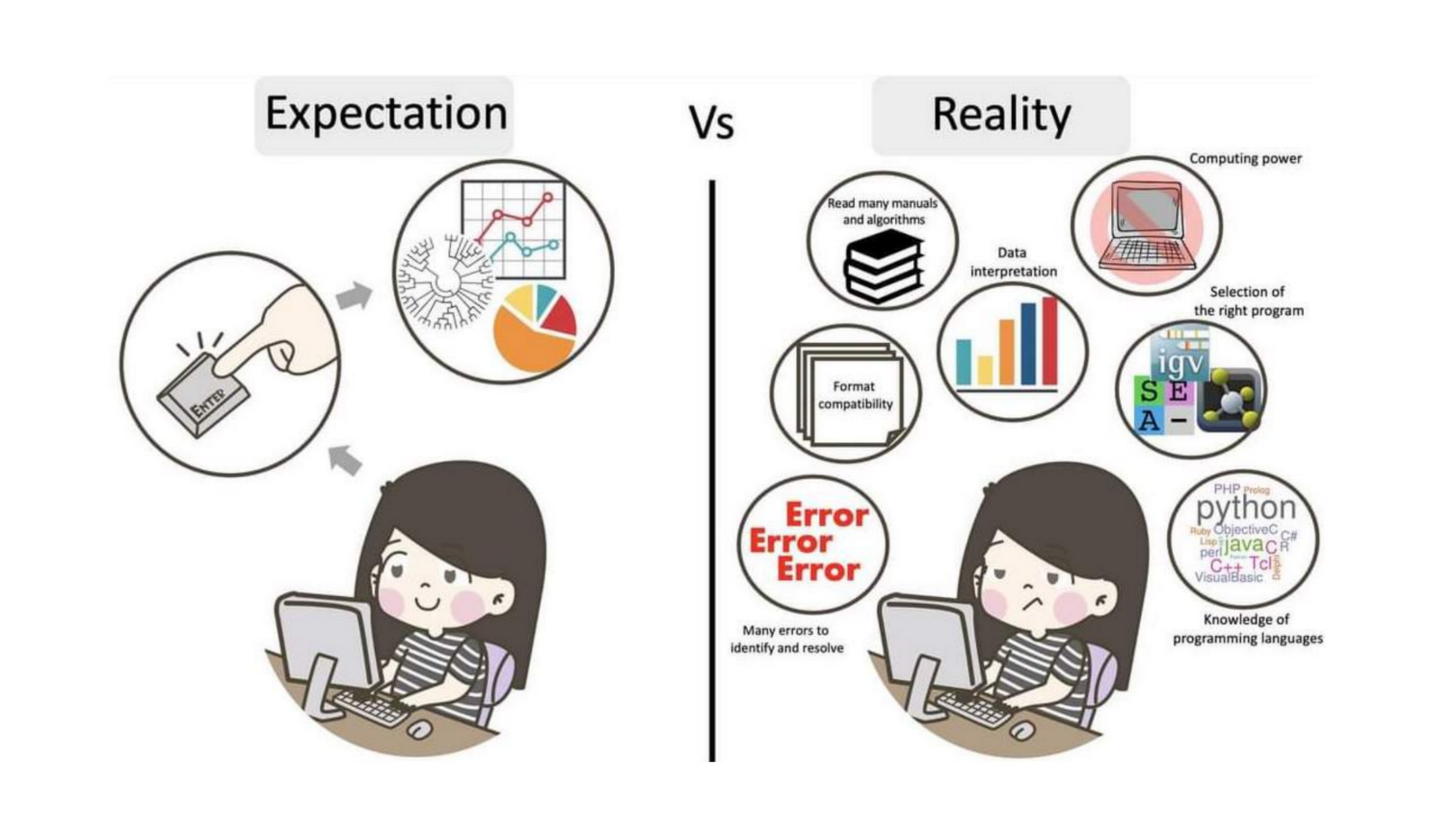
The truth about bioinformatics
Next generation Sequencing in a few slides
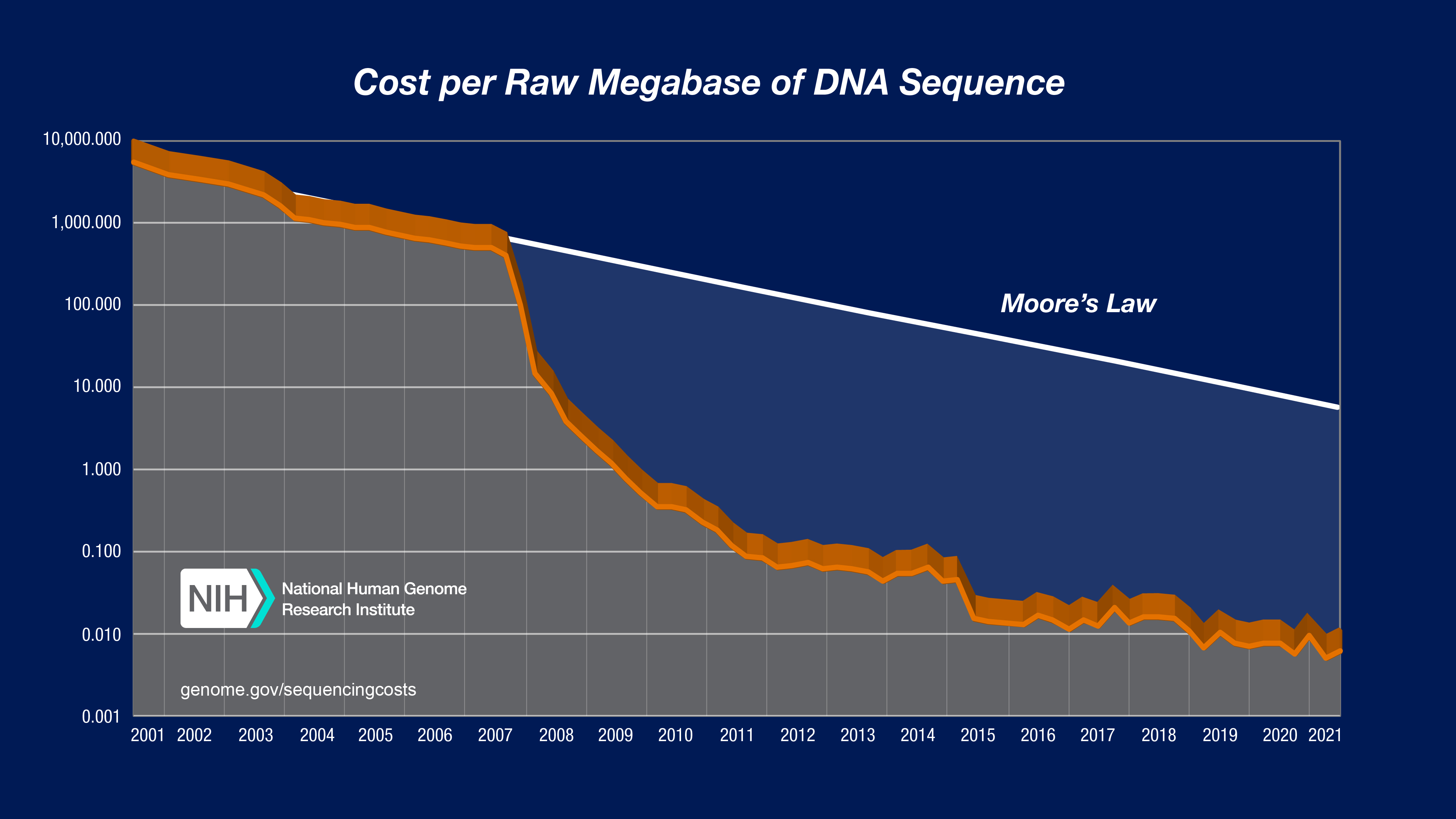
Sequencing Cost per Megabase
Genome Sequencing, why ?
Interest in a genome that has not yet been sequenced
- Assembly and annotation
- de novo sequencing
- chromosomal rearrangements
- metagenomics
Genome Sequencing, why ?
A reference genome is available
- Alignment (mapping) of reads on the genome
- Detection of genomic variants (SNPs)
- RNA-seq (gene expression)
- ChIP-seq (regulation of gene expression)
- Chromosomal rearrangements, variation in gene copy number
- Detection of small non-coding RNAs
- metagenomics
Sequencing challenges
- Smallest known (non viral) genome:
- Carsonella ruddii = 0.16 Mbp
- Largest known genome:
- Paris japonica = 150 Gbp
- Amoeba dubia = 670 Gbp
Sequencing challenges
- Maximum Reads Size :
- 1st generation (Sanger): up to 900 bp
- 2nd generation: up to 500 bp
- 3rd generation: up to 100 - 1000 Kbp
Need to cut the genome into millions of fragments (shotgun sequencing) from the 2 DNA strands.
The operation to reconstruct the genetic elements from the raw reads is called assembly.
Sequencing technologies
- First generation :
- Sanger sequencing
- First step : fragment cloning
- Reads up to 900 bp
- Expensive
- low throughput
- Sanger sequencing
Next generation Sequencing technologies
Second generation (since 2007)
- 454 - Sequencing by Synthesis - PCR Amplification
- SOLiD : Sequencing by Ligation - PCR Amplification
- Ion Torrent : Sequencing by Synthesis - PCR Amplification
- Illumina : Sequencing by Synthesis - PCR Amplification
Illumina : principles
- Based on “reversible terminated chemistry” : reversible terminators that enable the identification of single nucleotides as they are washed over DNA strands.
Three steps :
- Amplification of DNA fragments
- Sequencing
- Analysis
Prepare genomic DNA samples
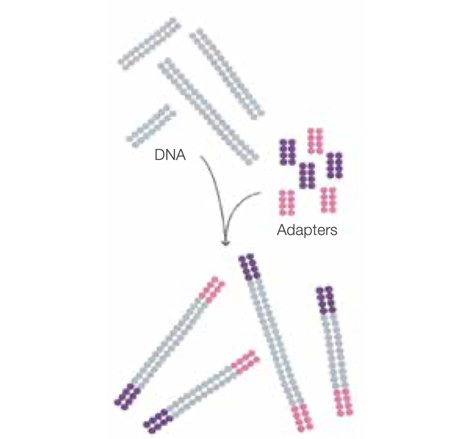
Randomly fragment genomic DNA and ligate adapters to both ends of the fragments
Attach DNA to Flow Cell Surface
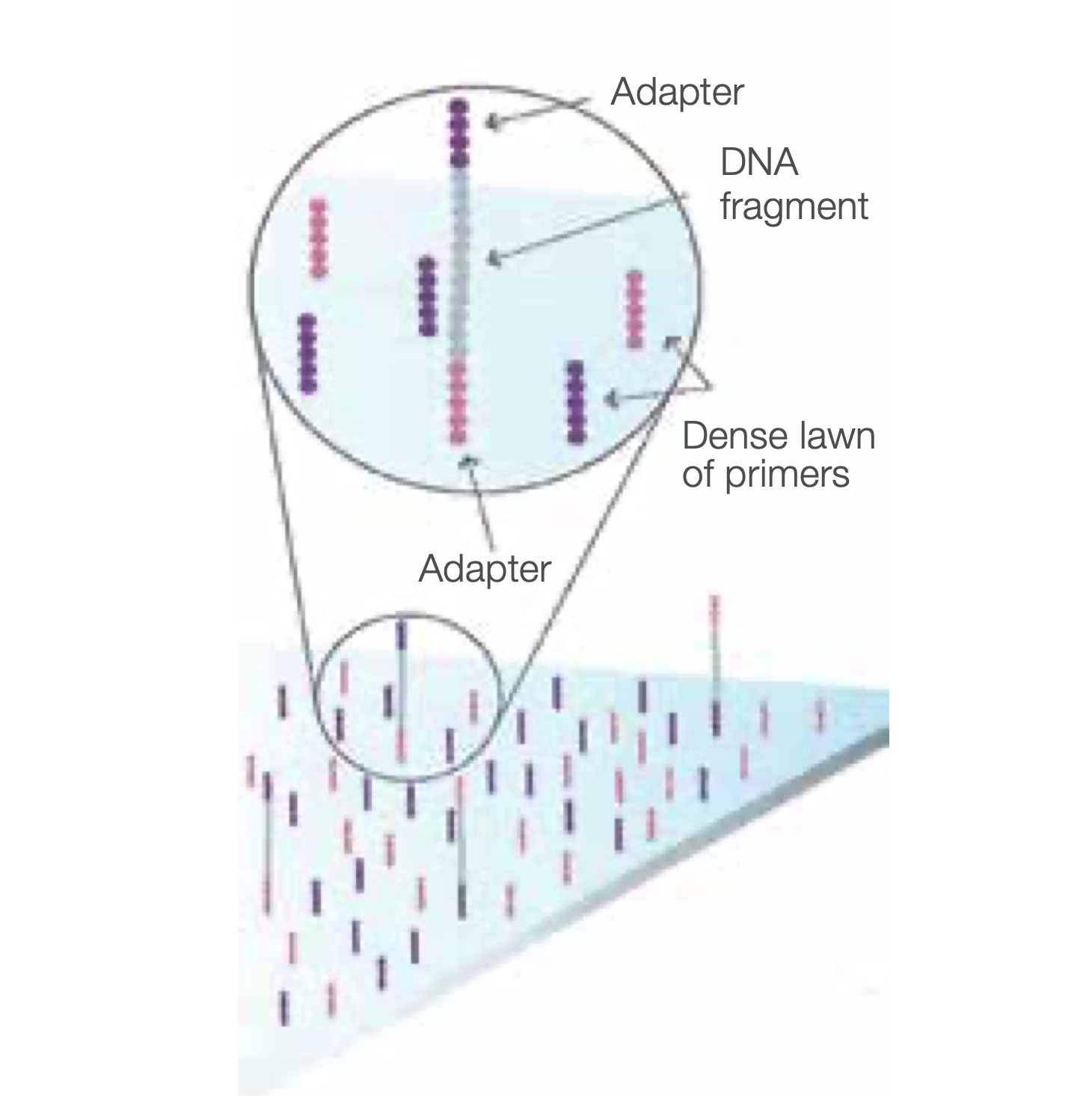
Bind single-stranded fragments randomly to the inside surface of the flow cell channels.
Bridge Amplification
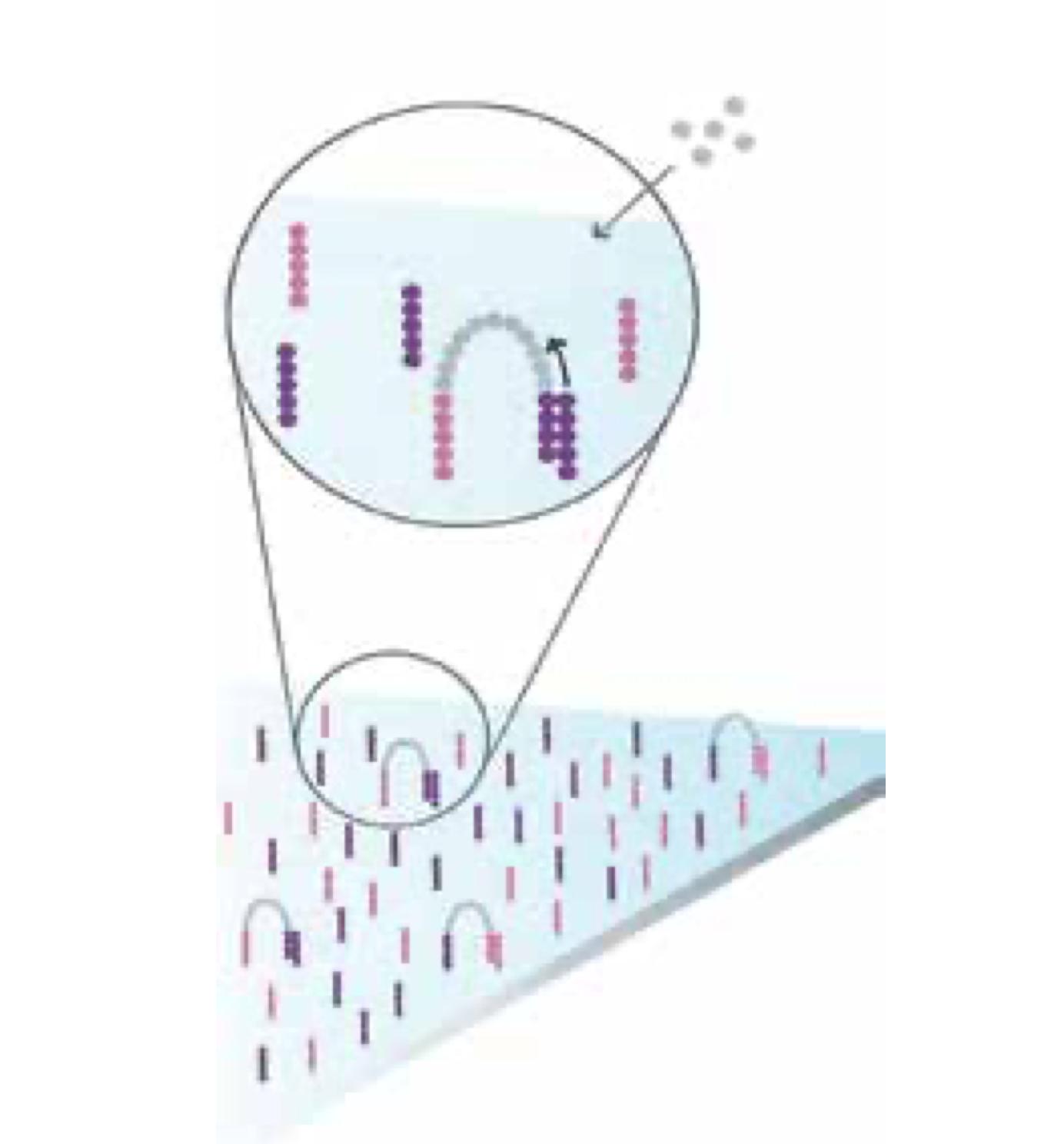
Add unlabelled nucleotides and enzyme to initiate solid-phase bridge amplification.
Fragments Become Double Stranded
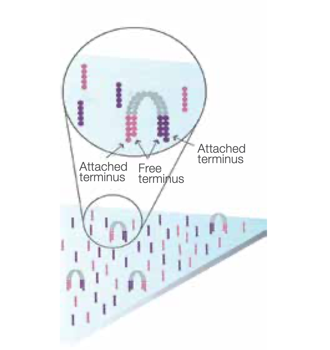
The enzyme incorporates nucleotides to build double-stranded bridges on the solid-phase substrate.
Denature the Double-Stranded Molecule
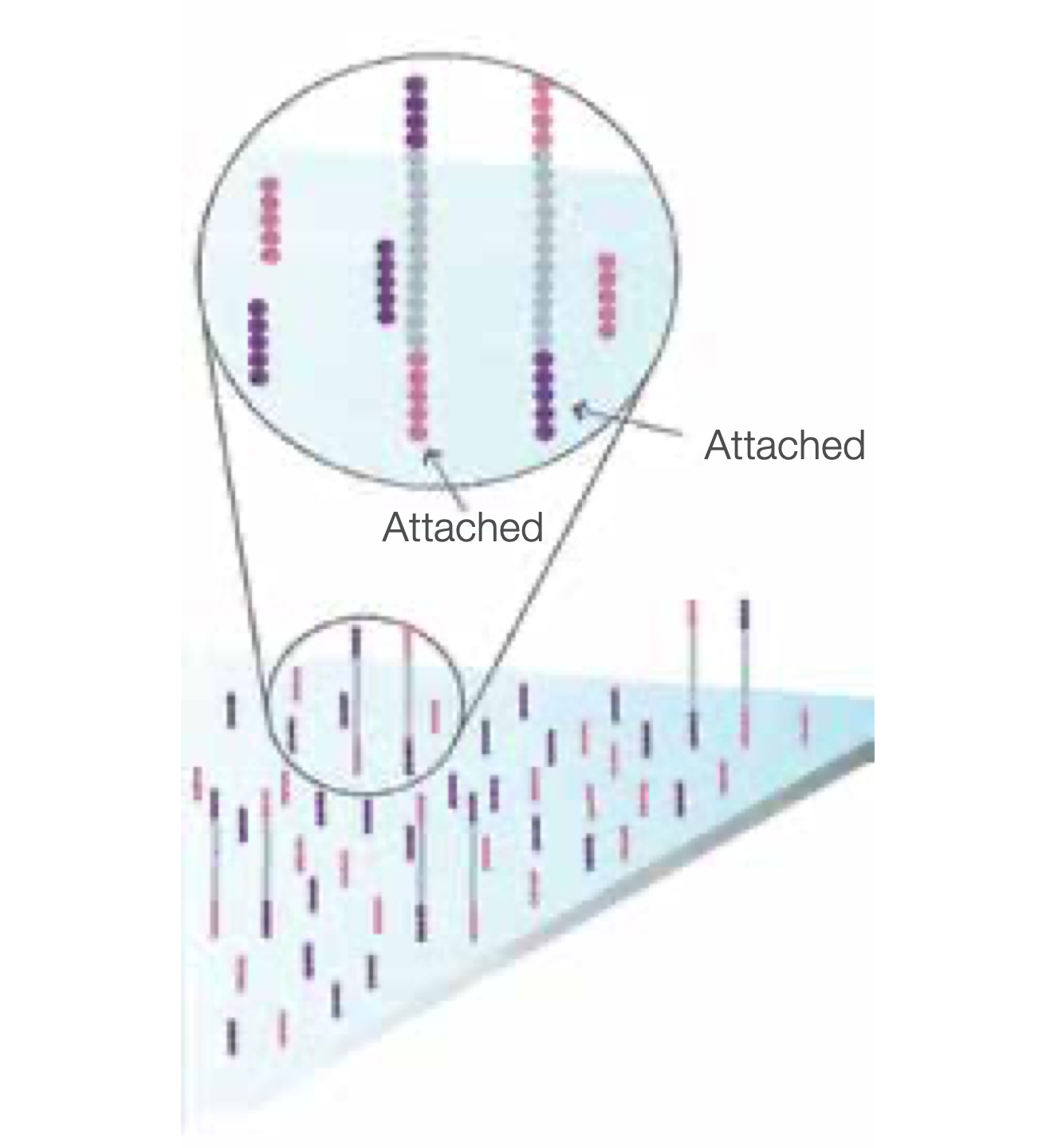
Denaturation leaves single-stranded templates anchored to the substrate.
Complete Amplification
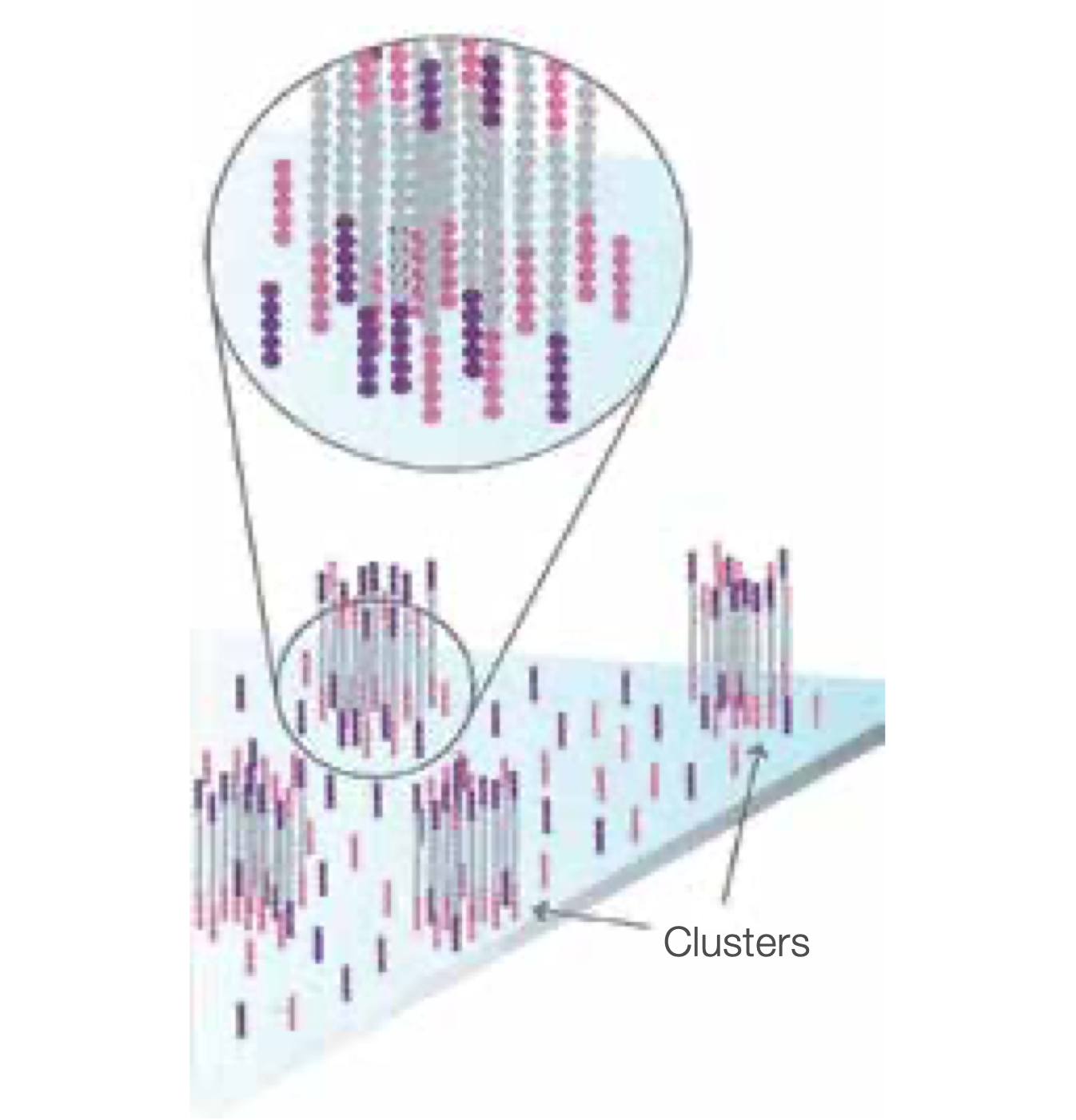
Several millions dense clusters of double-stranded DNA are grated in in channel of the flow cell.
Determine First Base
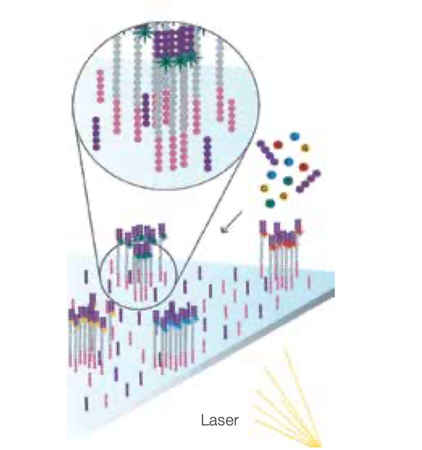
The first sequencing cycle begins by adding four labelled reversible terminators, primers, and DNA polymerase.
Image First Base
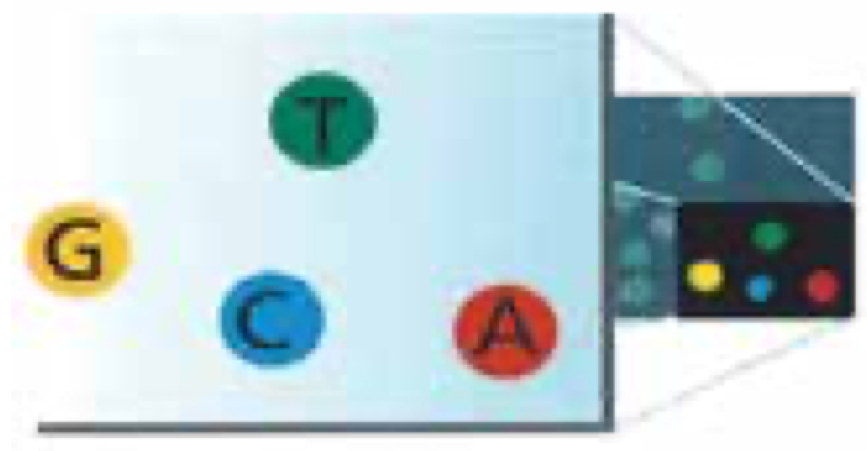
After laser excitation, the emitted fluorescence from each cluster is captured and the first base is identified.
The blocked 3’ terminus and florphore are removed,flow cell washed, leaving the terminator free for a second cycle.
Determine Second Base
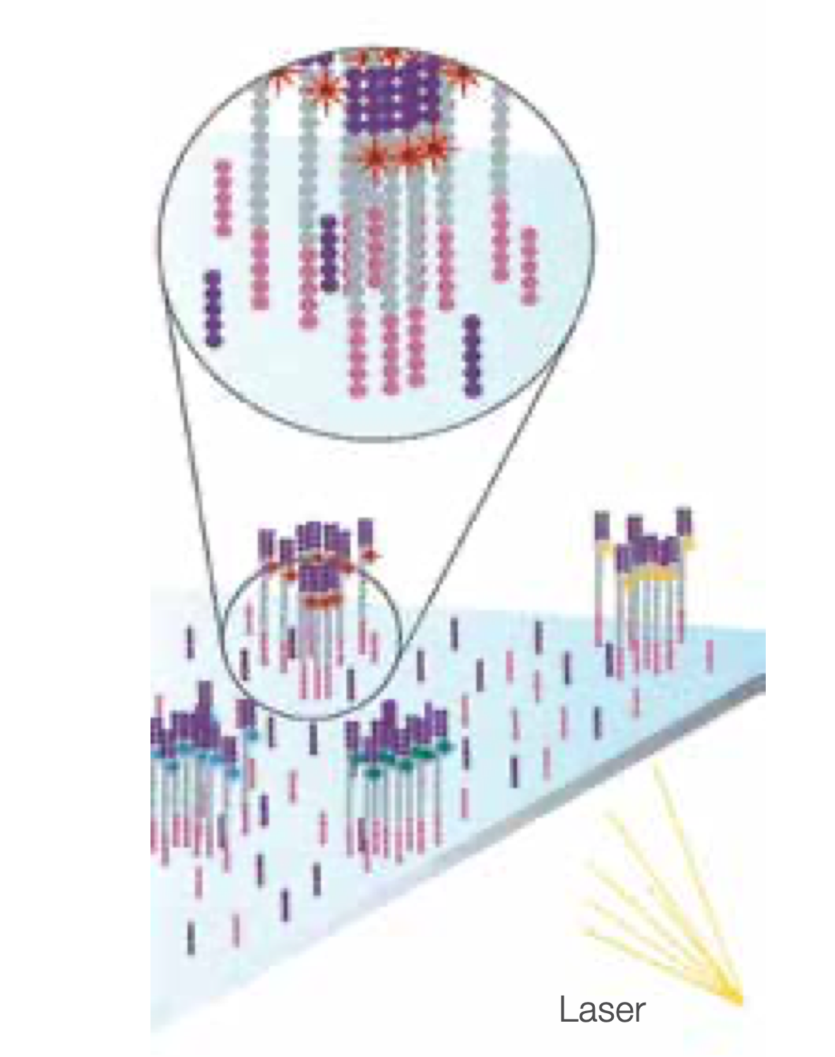
The next cycle repeats the incorporation of four labelled reversible terminators, primers, and DNA polymerase.
Image Second Chemistry Cycle
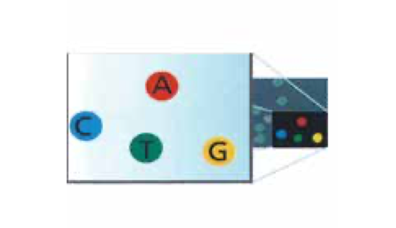
After laser excitation, the image is captured as before, and the identity of the second base is recorded.
Sequencing Over Multiple Chemistry Cycles
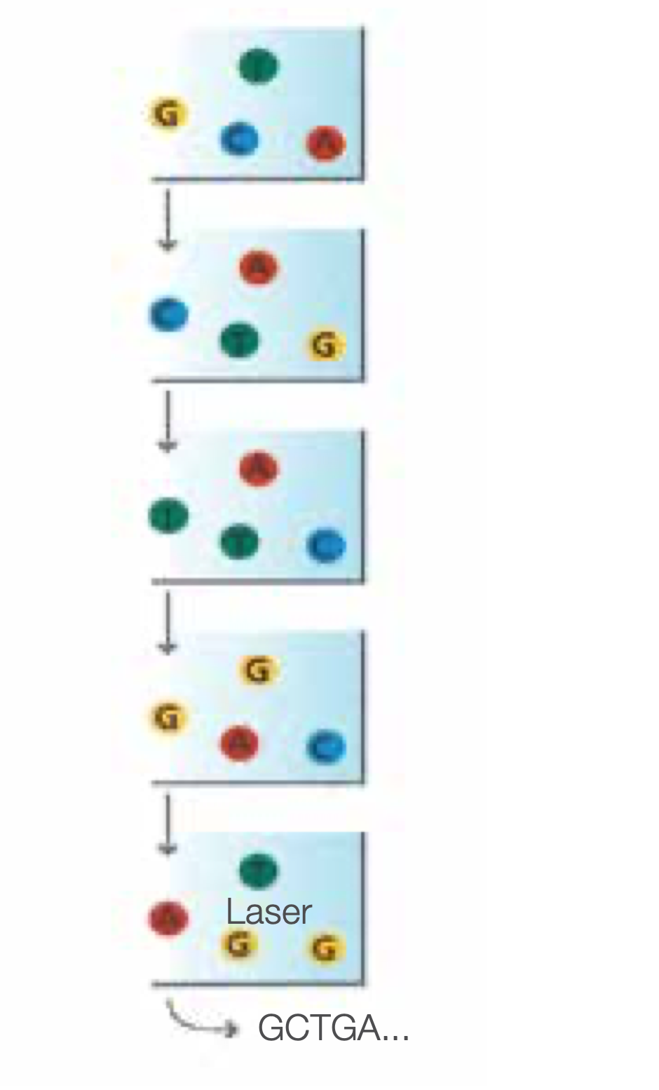
The sequencing cycles are repeated to determine the sequence of bases in a fragment, one base at a time.
Millions of clusters are processed in parallel, allowing high-throughput sequencing.
Illumina : summary
- High precision >99.5% (main type or errors : substitutions)
- Short reads (maximum 2 x 300)
- Huge throughput (up to 6 Tbp per run on NovaSeq)
- Some under-representation of rich AT- and GC- regions.
Sequencing - Vocabulary
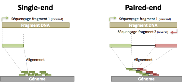
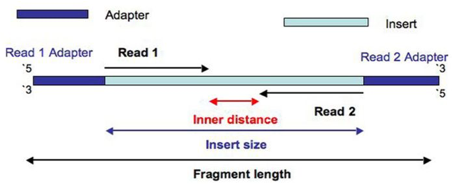
- Read: piece of sequenced DNA
- DNA fragment: 1 or more reads depending on whether the sequencing is single- or paired-end
- Insert: Fragment size
- Depth: \(\frac{N * L}{G}\)
\(N =\) number of reads
\(L =\) reads size
\(G =\) genome size - Coverage: % of genome covered

3d generation
Target the weaknesses of the 2nd generation :
- PCR amplification
- Short reads
Two main competitors (in production ) :
- Pacific Bioscience (PacBio)
- Oxford Nanopore Technologies (ONT)
PacBio

A polymerase is immobilized at the bottom of a sequencing unit called zero-mode waveguide (ZMW) .Four fluorescent-labelled nucleotides, which generate distinct emission spectrums, are added to the SMRT cell. As a base is held by the polymerase, a light pulse is produced that identifies the base. The replication processes in all ZMWs of a SMRT cell are recorded by a “movie” of light pulses, and the pulses corresponding to each ZMW can be interpreted to be a sequence of bases.
PacBio : summary
- Long reads (up to Kbs with SequelII)
- Depends on DNA quality
- High error rate. Tend to lower with depth
- Medium throughput
Applications :
- IsoSeq (RNA Isoform full length sequencing)
- Detection of DNA modification
- Assembly
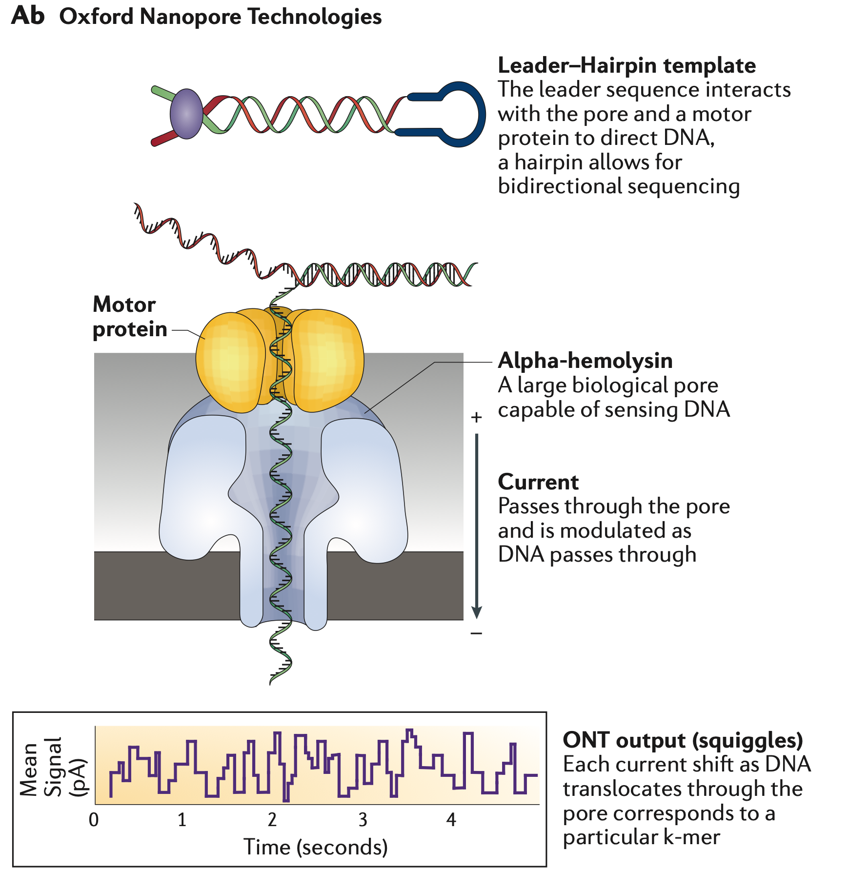
Oxford Nanopore

Oxford Nanopore
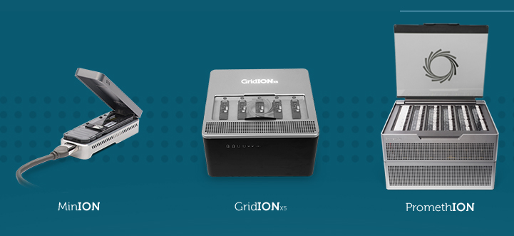
MinION, GridION, PromethION
Sequencing on The ISS

ONT Summary
- Ultra long reads ( up to 1 Mb (!) )
- Length of the reads depends on DNA quality
- Low to high throughput
- “On field” sequencing
- Direct RNA sequencing, peptide sequencing
- High error rate (5-10%), tends to lower with new chemistry, base calling algorithms and depth
ONT Applications
- Full length isofrom sequencing, direct RNA sequencing
- Detection of DNA modification
- Assembly
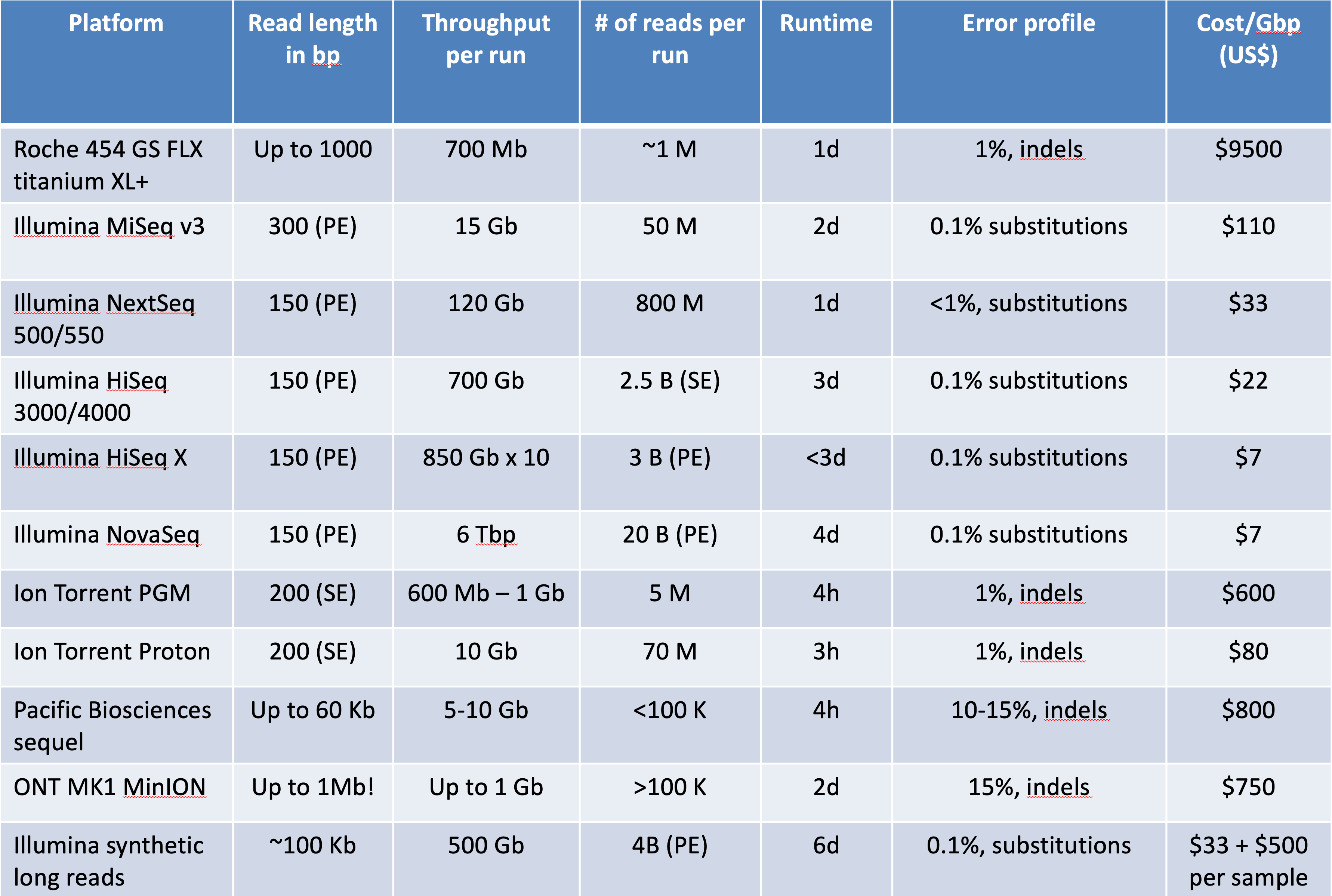
An other view on sequencing technologies (probably out of date)
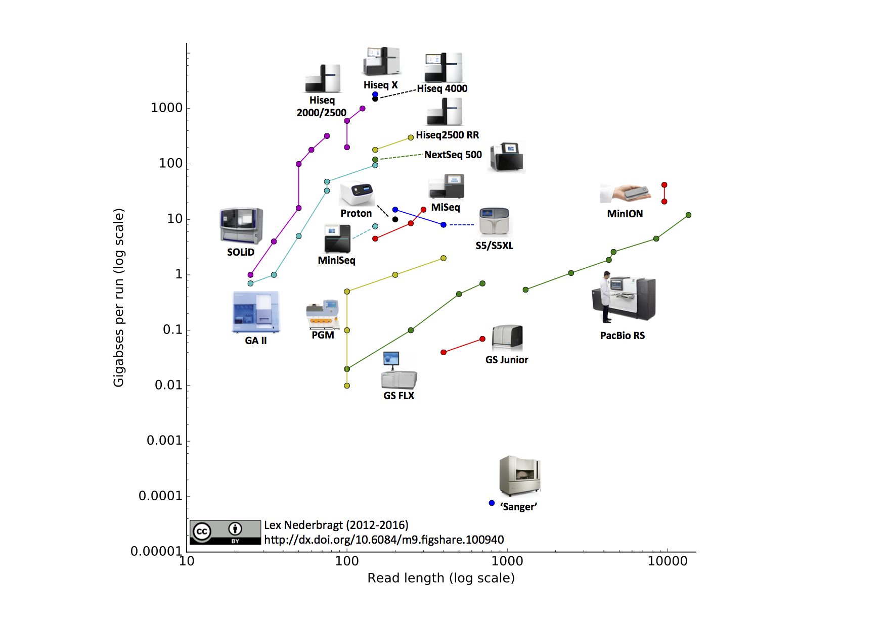
Global Summary (probably out of date)
An interesting review [1]
Nature review : Milestones in Genomic Sequencing
Connect to Galaxy
Practical session :
- Escherichia coli genome (re)sequencing
- Illumina MiSeq
- Paired-end sequencing (2*150bp , insert size ~300bp)
- Sub-sampled
Connect to Galaxy
https://galaxy.migale.inrae.fr
Login : stageXX
Data in
Shared Data / Data Libraries / formation NGS / ReadsReferences in
Shared Data / Data Libraries / formation NGS / Refs
FASTQ format
FASTQ syntax
The FASTQ format is the de facto standard by which all sequencing instruments represent data. It may be thought of as a variant of the FASTA format that allows it to associate a quality measure to each sequence base: FASTA with QUALITIES.
FASTQ format consists of 4 sections:
- A FASTA-like header, but instead of the
>symbol it uses the@symbol. This is followed by an ID and more optional text, similar to the FASTA headers. - The second section contains the measured sequence (typically on a single line), but it may be wrapped until the
+sign starts the next section. - The third section is marked by the
+sign and may be optionally followed by the same sequence id and header as the first section - The last line encodes the quality values for the sequence in section 2, and must be of the same length as section 2.
FASTQ syntax
FASTQ quality
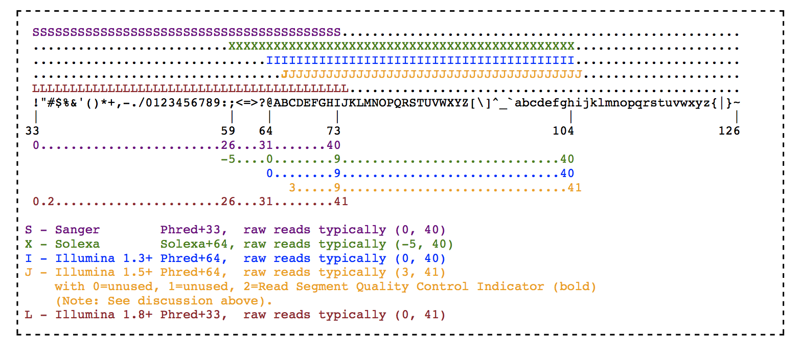
Each character represents a numerical value: a so-called Phred score, encoded via a single letter encoding.
The numbers represent the error probabilities via the formula: \(Error=10^{-P/10}\)
It is basically summarized as:
- P=0 means 1/1 (100% probability of error)
- P=10 means 1/10 (10% probability of error)
- P=20 means 1/100 (1% probability of error)
- P=30 means 1/1000 (0.1% probability of error)
- P=40 means 1/10000 (0.01% probability of error)
FASTQ quality encoding specificities
There was a time when instrumentation makers could not decide at what character to start the scale. The current standard shown above is the so-called Sanger (+33) format where the ASCII codes are shifted by 33. There is the so-called +64 format that starts close to where the other scale ends.
FASTQ Header informations
Information is often encoded in the “free” text section of a FASTQ file.
EAS139: the unique instrument name136: the run idFC706VJ: the flowcell id2: flowcell lane2104: tile number within the flowcell lane15343: ‘x’-coordinate of the cluster within the tile197393: ‘y’-coordinate of the cluster within the tile1: the member of a pair, 1 or 2 (paired-end or mate-pair reads only)Y: Y if the read is filtered, N otherwise18: 0 when none of the control bits are on, otherwise it is an even numberATCACG: index sequence
This information is specific to a particular instrument/vendor and may change with different versions or releases of that instrument.
Fastq import & visualisation
Quality control
Why QC’ing your reads ?
What are the information you want to know about the sequencing when you perform Quality Control ?
Collective Answer on this collaborative whiteboard
Why QC’ing your reads ?
Try to answer to (not always) simple questions:
Quality control
- Are data conform to the expected level of performance?
- Size
- Number of reads
- Quality
- Residual presence of adapters or indexes ?
- Are there (un)expected technical biases
- Are there (un)expected biological biases
Warning
Quality control without context leads to misinterpretation
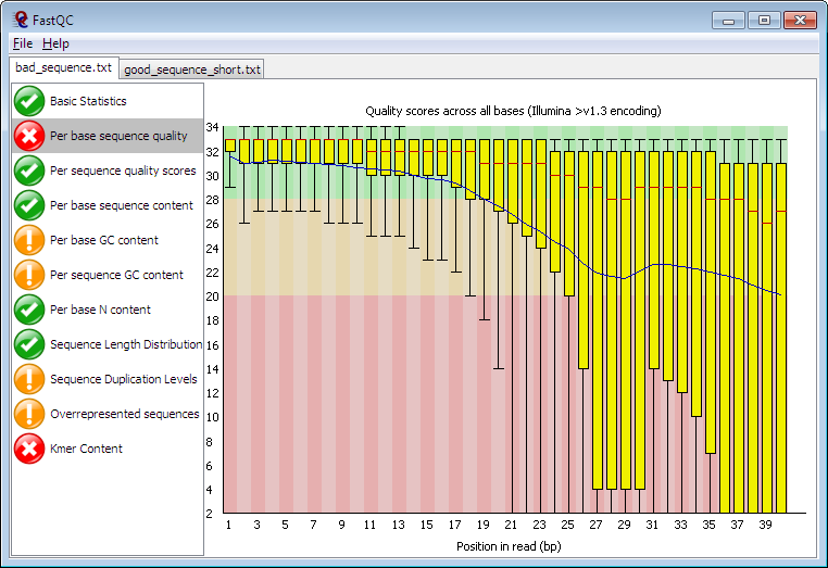
Quality control for FASTQ files : FastQC [2]
- QC for (Illumina) FastQ files
- Command line fastqc or graphical interface
- Complete HTML report to spot problem originating from sequencer, library preparation, contamination
- Summary graphs and tables to quickly assess your data
Quality Control with FastQC
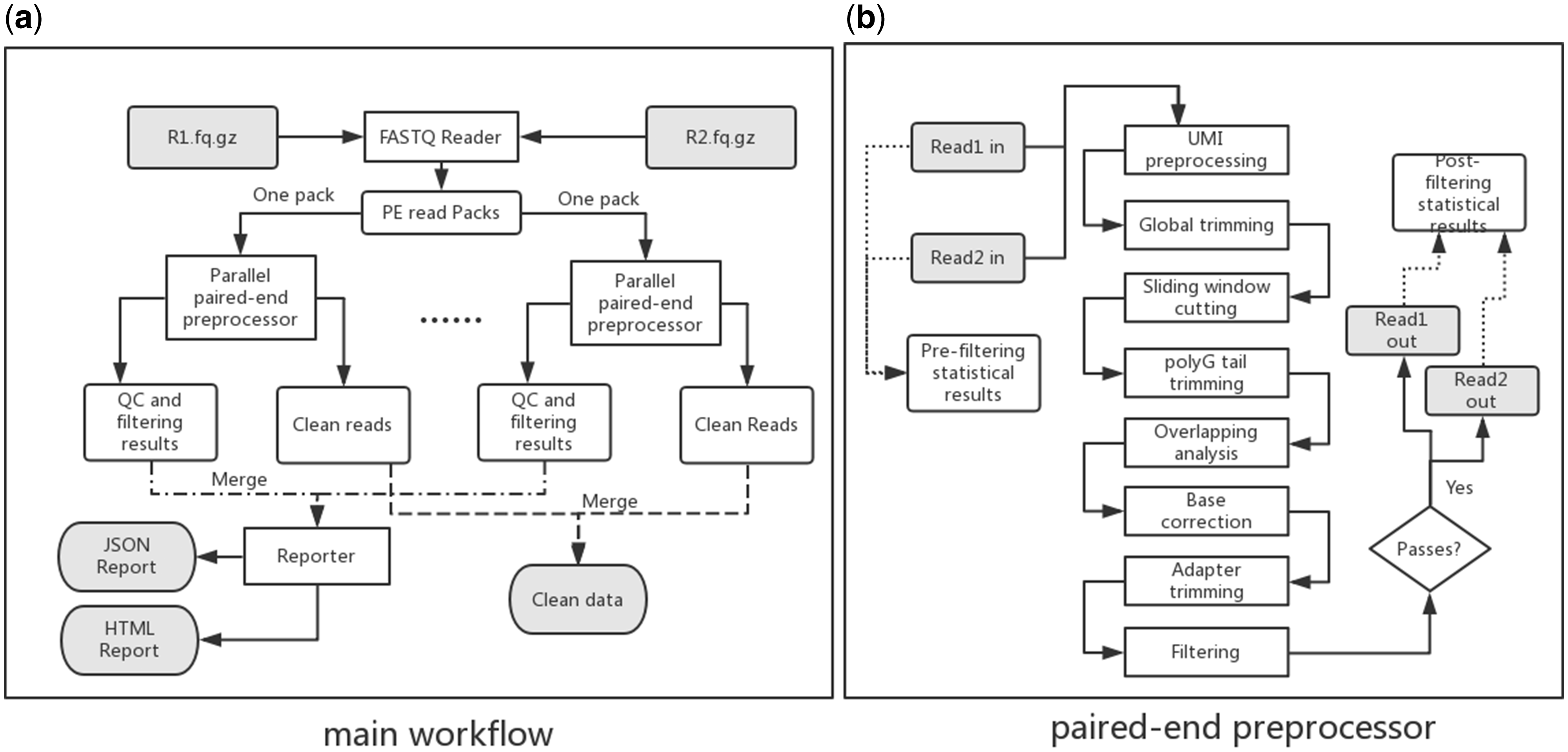
Reads cleaning
Objectives
- Detect and remove sequencing adapters (still) present in the FastQ files
- Filter / trim reads according to quality (as plotted in FastQC)
Tools
- Simple & fast :
Sickle[3] (quality) - dedicated to adapters
cutadapt[4] (adpater removal) - Ultra-configurable :
Trimmomatic - All in one & ultra-fast :
fastp[5]
Clean your data with Fastp
Assembly
Assembly : principles
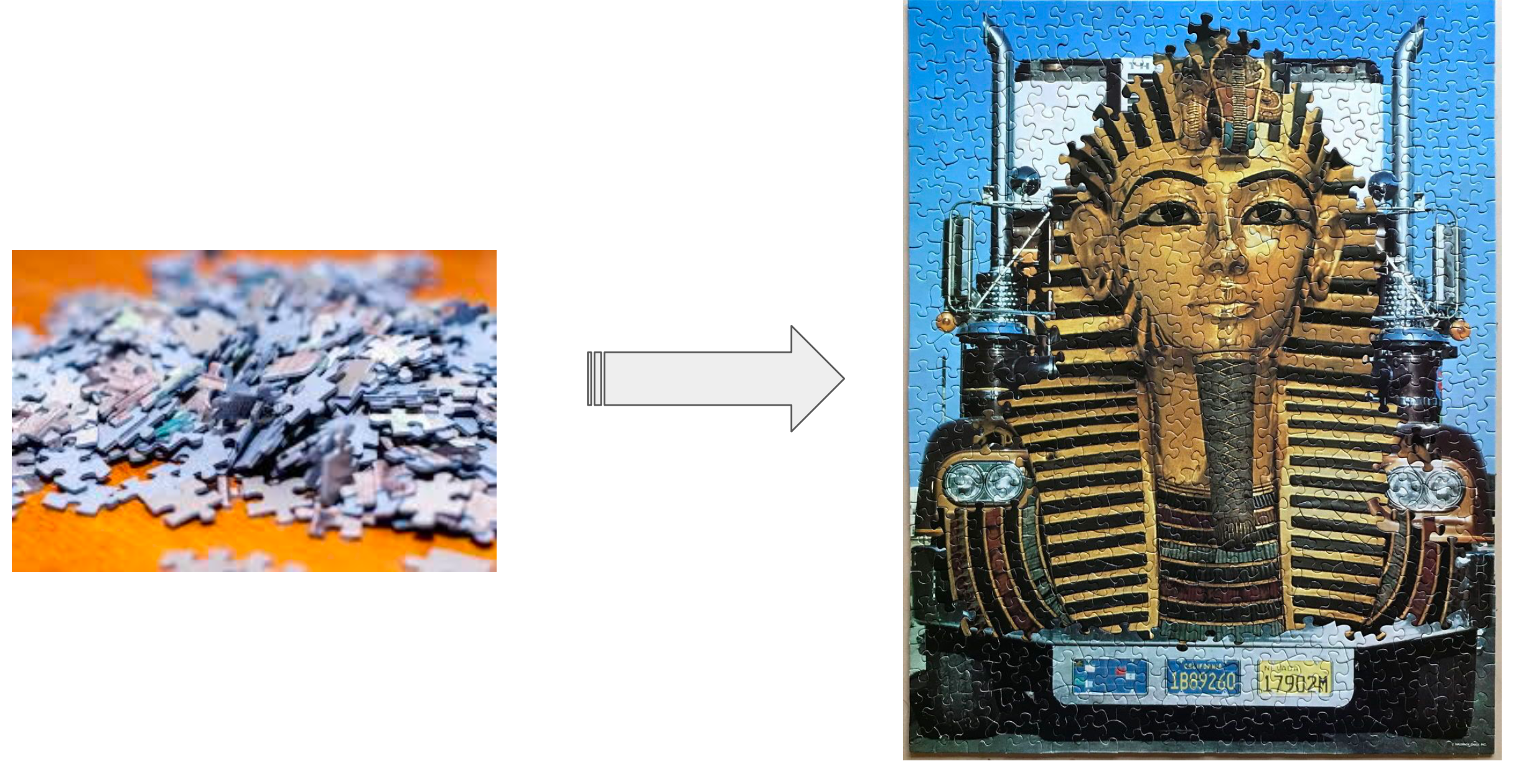
Similar to a puzzle :
- millions of pieces
- without the original image
- with pieces in both sense
- the pieces do not necessarily fit together (sequencing errors)
- parts of the puzzle are missing (cover + sequencing bias)
Assembly
All assembly algorithms are based on read overlap.
Different ways of calculating overlap :
“All vs All” comparison :
- “old” assemblers based on this approach
- Graph representing overlap between reads
- Quadratic number of comparison (number of reads^2 )
- do not scale with billion of reads
de Bruijn Graph
- Named after Nicolaas Govert de Bruijn
- Directed graph representing overlaps between sequences of symbols
- Sequences can be reconstructed by moving between nodes in graph
De Bruijn Graph
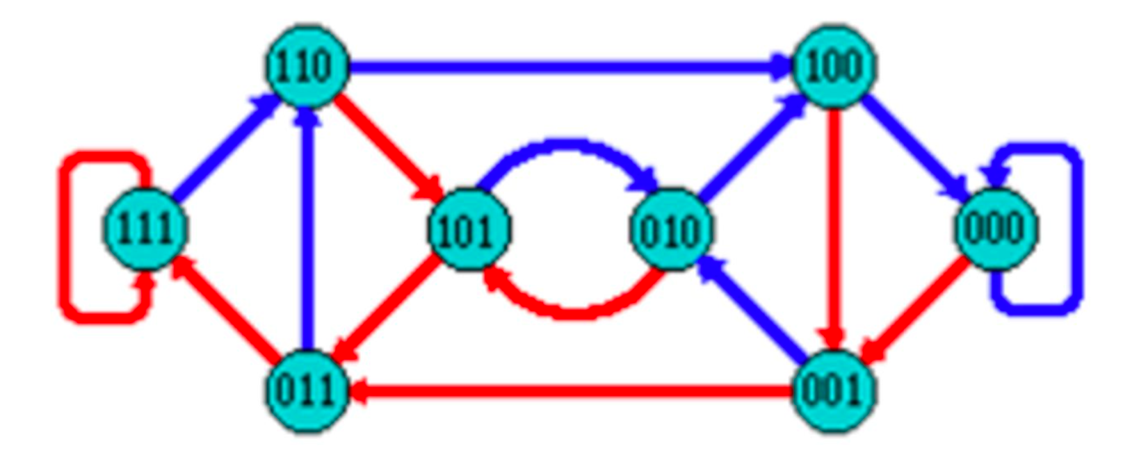
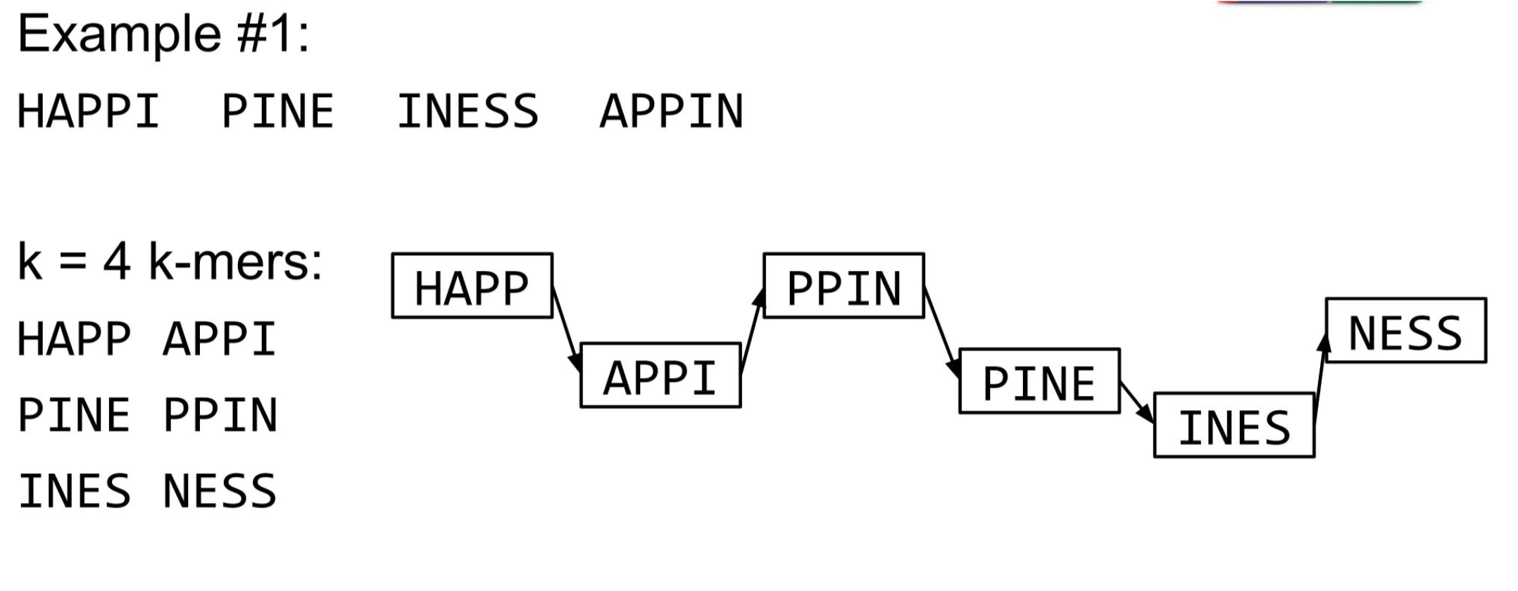
- A directed graph of sequences of symbols
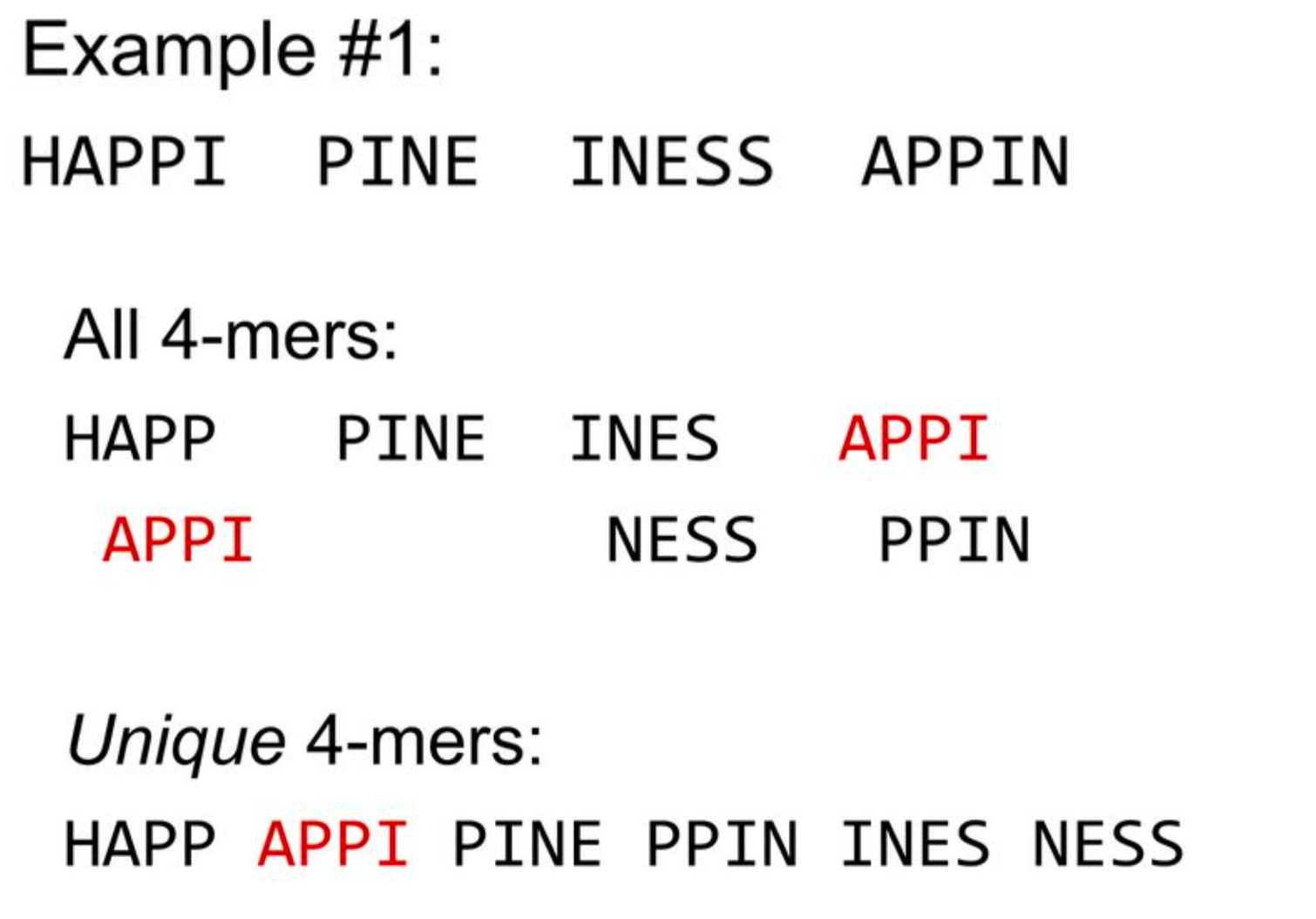
- Nodes in the graph are k-mers
- Edges represent consecutive k-mers (k-1 symbols overlap)
Consider the 2 symbol alphabet (0 & 1) de Bruijn Graph for k=3
Producing sequences
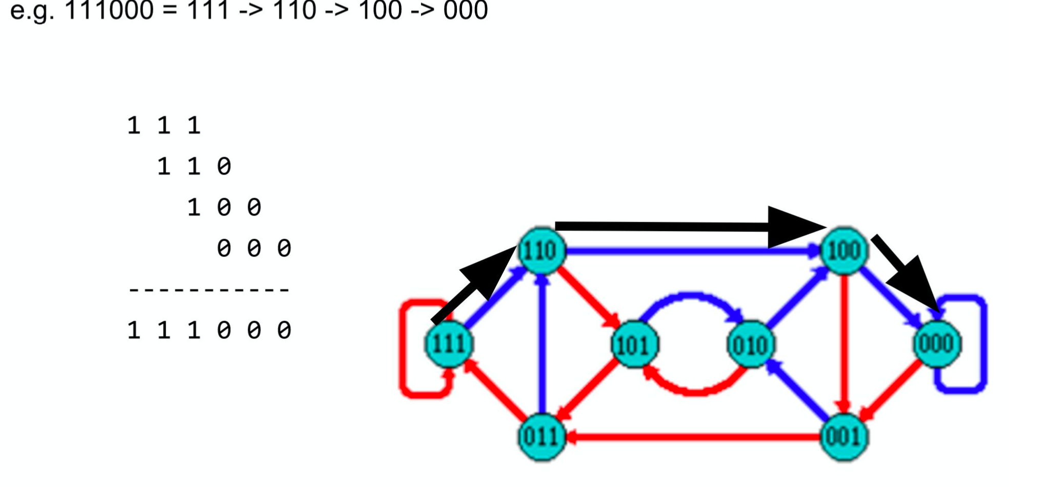
- Sequences of symbols are produced by moving through the graph
K-mers ?
- To be able to use de Bruijn graphs, we need reads of length L to overlap by L-1 bases.
- Not all reads will overlap another read perfectly.
- Read errors
- Coverage “holes”
- Not all reads are the same length (depending on technology and quality clean-up)
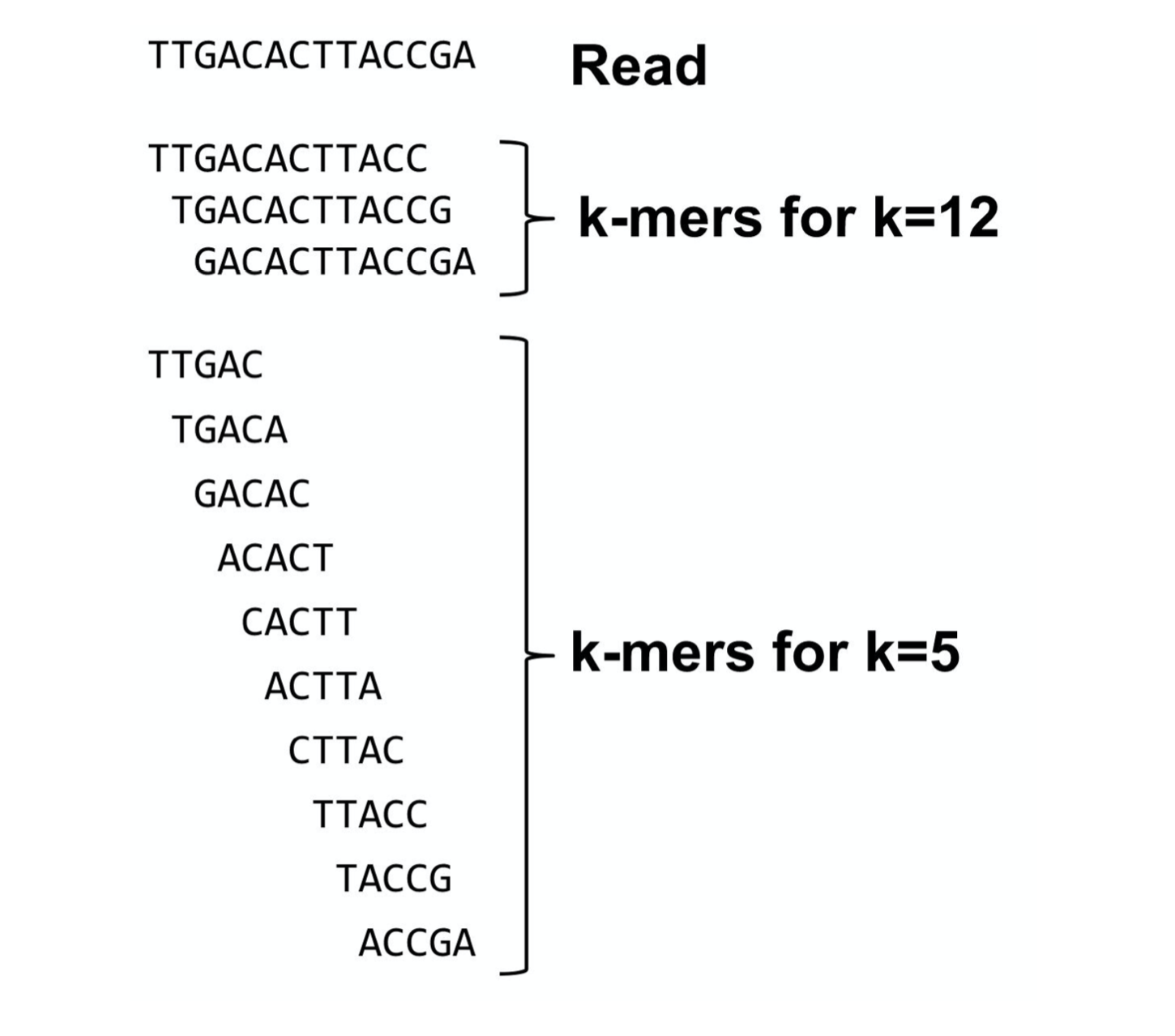
To help us get around these problems, we use all k-length subsequences of the reads, these are the k-mers.
What are K-mers ?
K-mers de Bruijn graph

K-mers de Bruijn graph
K-mers de Bruijn graph
The problem of repeats
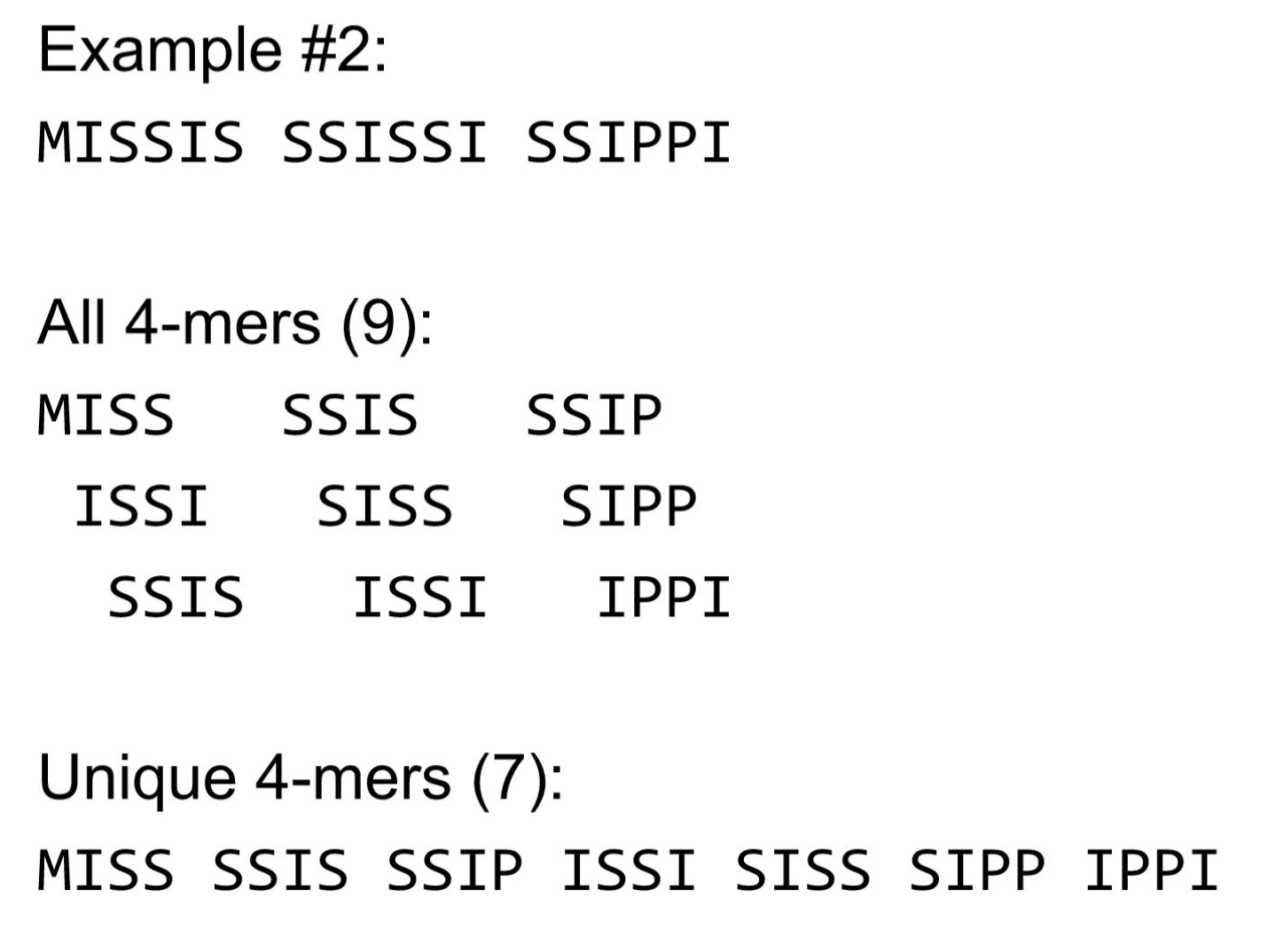
The problem of repeats
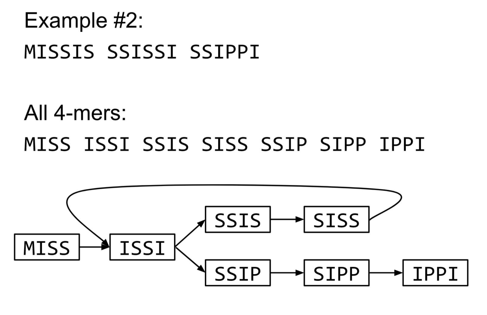
The problem of repeats
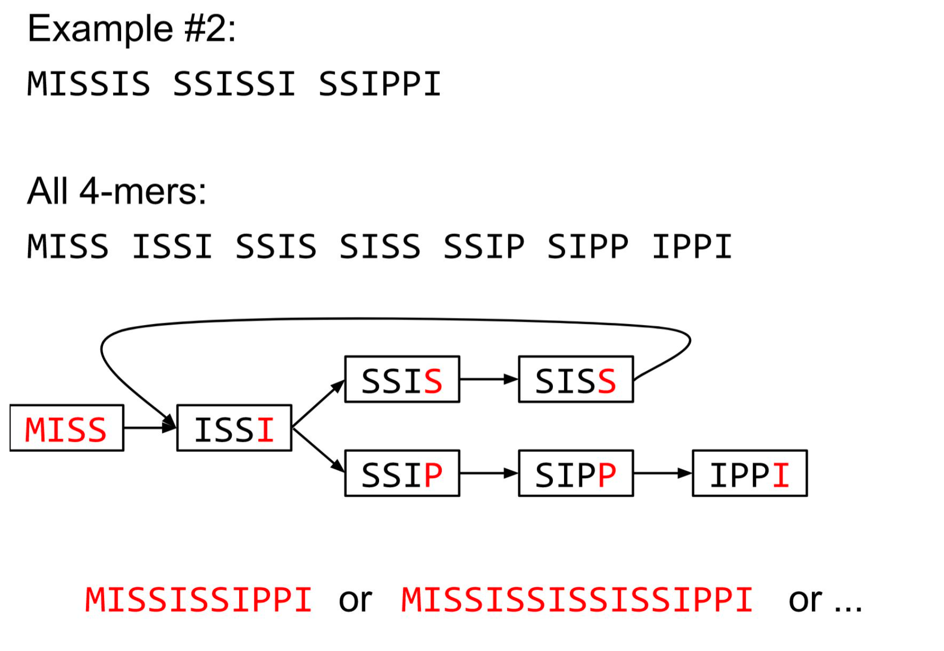
Different k
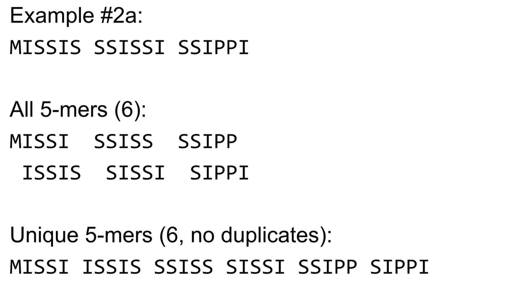
Different k
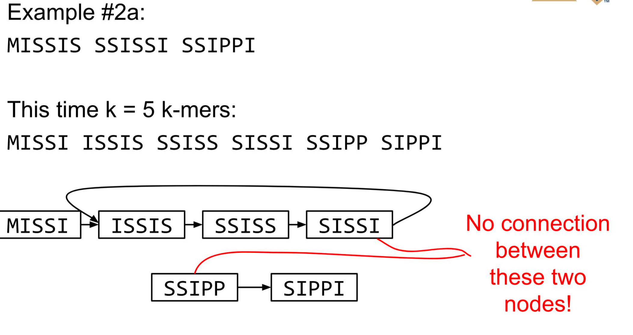
2 contigs : MISSISSIS & SSIPPI
Choose k wisely
- Lower k
- More connections
- Less chance of resolving small repeats
- Higher k-mer coverage
- Higher k
- Less connections
- More chance of resolving small repeats
- Lower k-mer coverage
Optimum value for k will balance these effects.
Sequencing errors
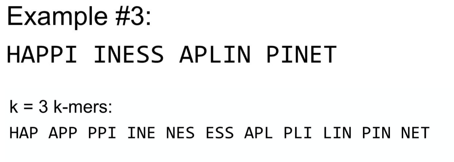
Sequencing errors
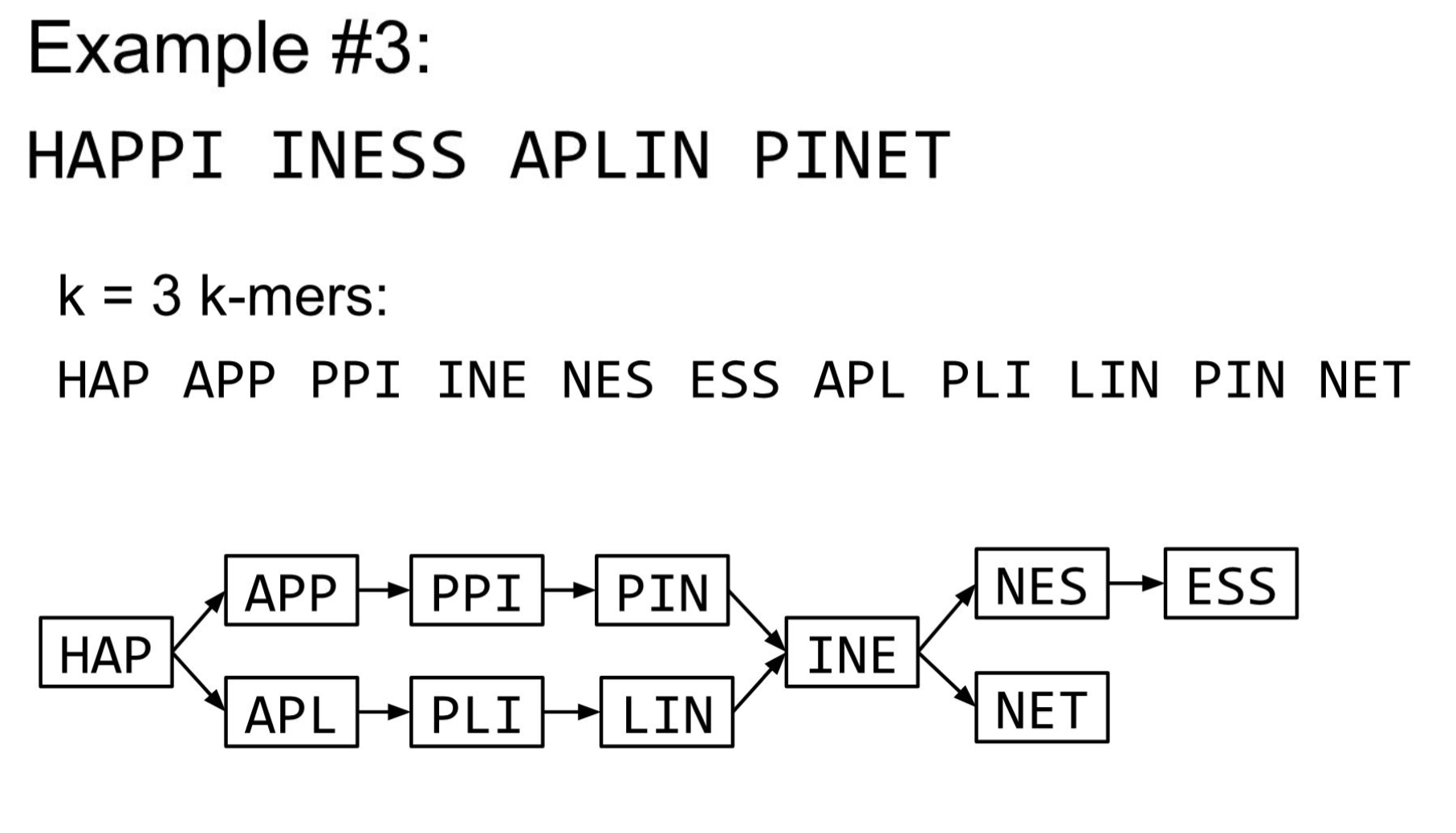
Sequencing errors
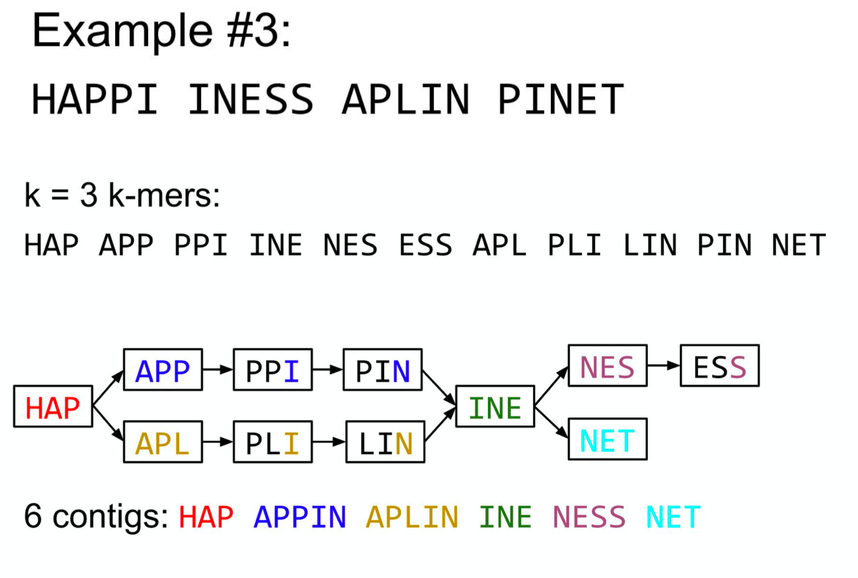
More coverage
- Errors won’t be duplicated in every read
- Most reads will be error free
- We can count the frequency of each k-mer
- Annotate the graph with the frequencies
- Use the frequency data to clean the de Bruijn graph
More coverage depth will help overcome errors!
Sequencing errors - coverage
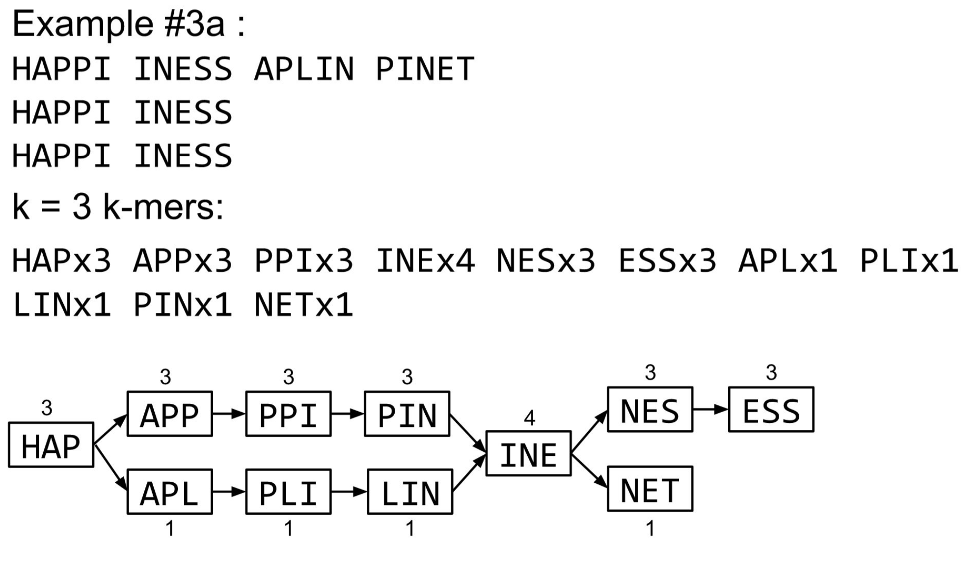
Which path looks most valid ? Why ?
An important parameter : coverage cutoff
- At what point is a low coverage indicative of an error?
- Can we ignore low coverage nodes and paths?
- This is a new assembly parameter
Coverage cut-off is an important parameter to differentiate error from real variations
de Bruijn Graph Assembly process
- Select a value for k
- “Hash” the reads (make the kmers)
- Count the kmers
- Make the de Bruijn graph
- Perform graph simplification steps - use cov cutoff
- Read off contigs from simplified graph
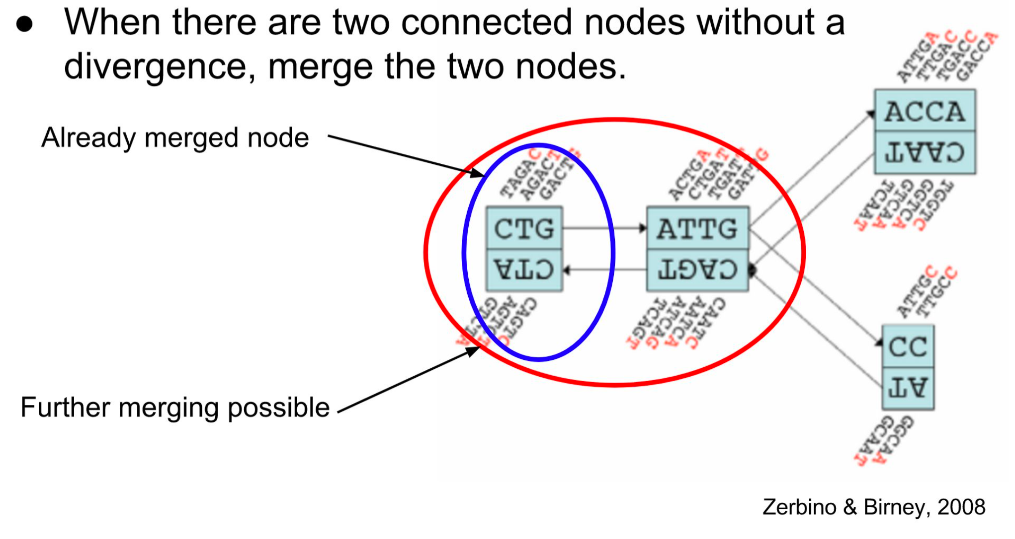
Graph simplification : Chain Merging
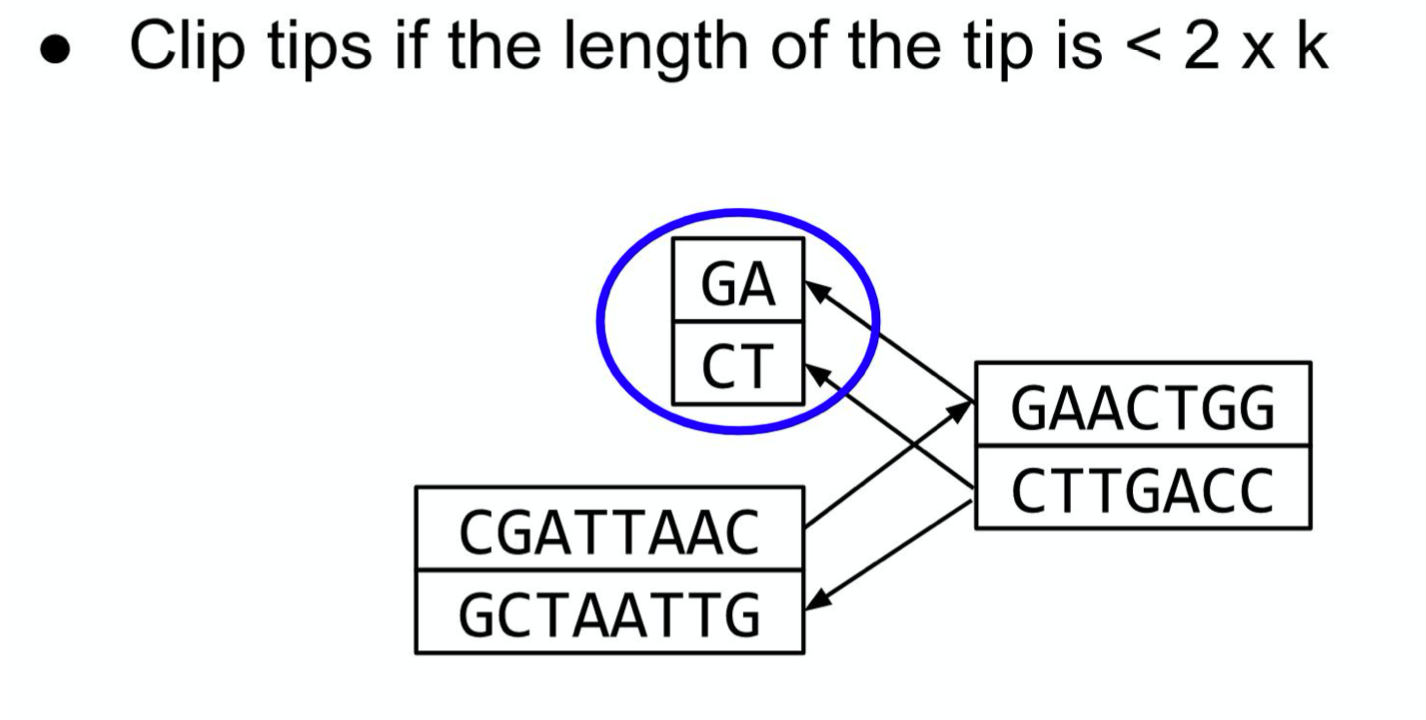
Graph simplification : Tip Clipping
Graph simplification : Bubble Collapsing
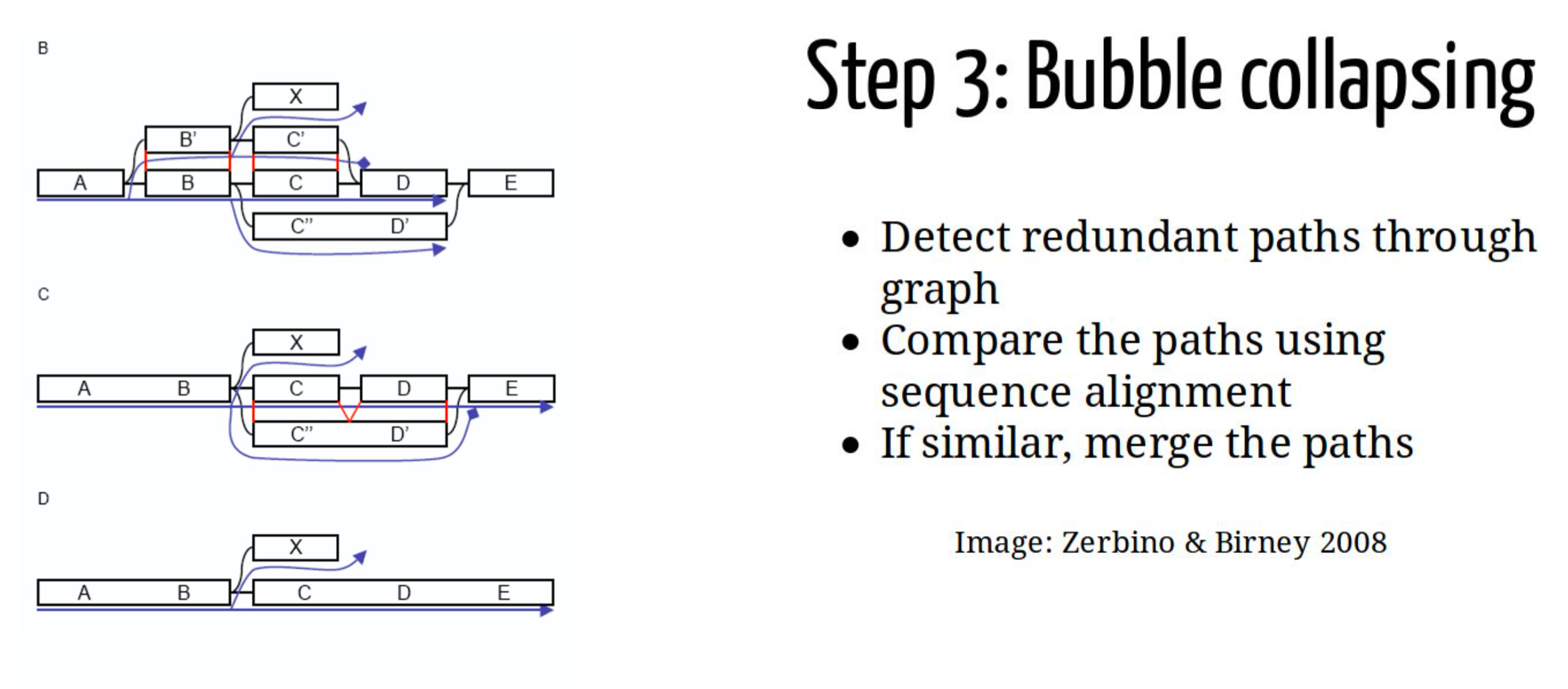
Make contigs
Find an unbalanced node in the graph
Follow the chain of nodes and “read off” the bases to produce the contigs
Where there is an ambiguous divergence/convergence, stop the current contig and start a new one.
Re-trace the reads through the contigs to help with repeat resolution
Graph simplification : Remove low coverage nodes
remove erroneous nodes and edges using the “coverage cutoff”
genuine short nodes will be kept because of their high coverage
Assemble with SPADES
SPADES [6] is the de Bruijn graph assembler by Pavel Pevzner’s group out of St. Petersburg
- Uses multiple k-mers to build the graph
- Graph has connectivity and specificity
- Usually use a low, medium and high k-mer size together.
- Performs error correction on the reads first
- Maps reads back to the contigs and scaffolds as a check
- Under active development
Assembly your data with SPADES
Assembly quality
QUAST
After assembly, we use QUAST [7] to evaluate and compare genome assemblies.
What QUAST does :
- De novo genome assembly evaluation
- Reference-based evaluation
- Evaluating so-called misassemblies
- Report and visualisation
De novo metrics
Evaluation of the assembly based on:
- Number of contigs greater than a given threshold (0, 1kb, …)
- Total / thresholded assembly size
- Largest contig size
- N50 : the sequence length of the shortest contig at 50% of the total assembly length, equivalent to a median of contig lengths. (N75 idem, for 75%)
- L50 : the number of contigs at 50% of the total assembly length. (L75 idem, for 75%)
Reference-based metrics
- Metrics based on based on an alignment of all contigs on a reference genome. :
- duplication rate
- percent genome complete
- NGA50 : equivalent of N50 but with the aligned block of the contigs
- “Misassemblies” : breakpoint of alignment in a contigs. ”
- Visualisation available
Assembly QC with Quast
Alignment
Alignment strategies
Global alignment
Global alignments, which attempt to align every residue in every sequence, are most useful when the sequences in the query set are similar and of roughly equal size. (This does not mean global alignments cannot start and/or end in gaps.) A general global alignment technique is the
Needleman–Wunsch algorithm, which is based on dynamic programming.
Alignment strategies
Local alignment
Local alignments are more useful for dissimilar sequences that are suspected to contain regions of similarity or similar sequence motifs within their larger sequence context. The
Smith–Waterman algorithmis a general local alignment method based on the same dynamic programming scheme but with additional choices to start and end at any place.
Seed-and-extend for NGS data

Seed-and-extend for NGS data
Seed-and-extend mappers are a class of read mappers that break down each read sequence into seeds (i.e., smaller segments) to find locations in the reference genome that closely match the read.
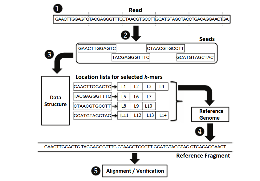
- The mapper obtains a read
- The mapper selects smaller DNA segments from the read to serve as seeds
- The mapper indexes a data structure with each seed to obtain a list of possible locations within the reference genome that could result in a match
- For each possible location in the list, the mapper obtains the corresponding DNA sequence from the reference genome
- The mapper aligns the read sequence to the reference sequence, using an expensive sequence alignment algorithm to determine the similarity between the read and the reference.
Mapping
- For further analysis it is necessary to map all the reads on the contigs.
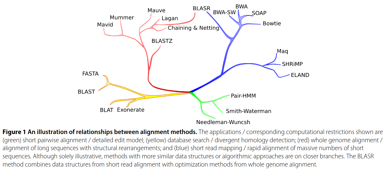
Mapping
BAM/SAM
SAM= Sequence Alignment MapBAM= Binary Alignment Map
These files represent an alignment of FASTQ reads against a reference like a FASTA.
- After a header section (for reference), each line represents the alignment of one read.
BAM/SAM
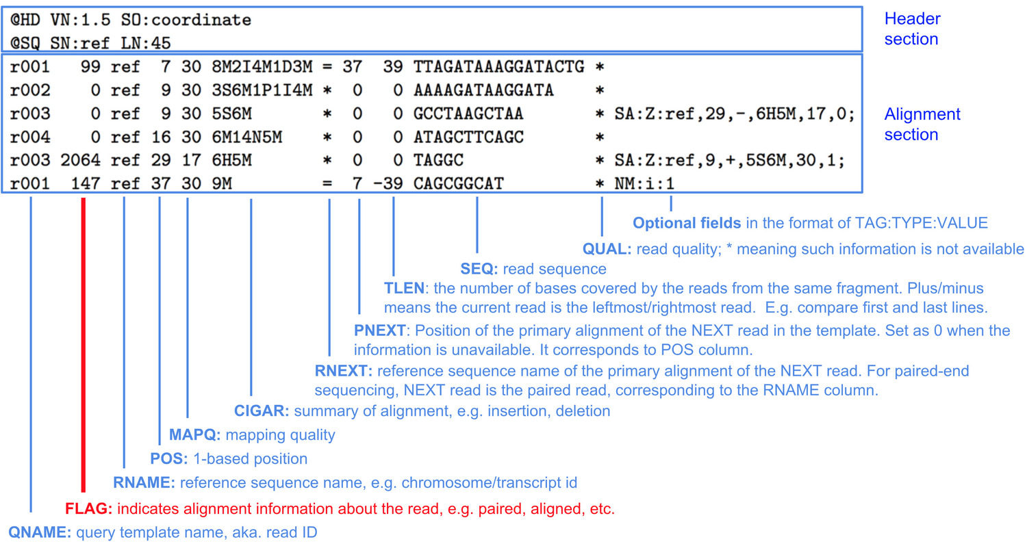
Mapping
Vizualisation
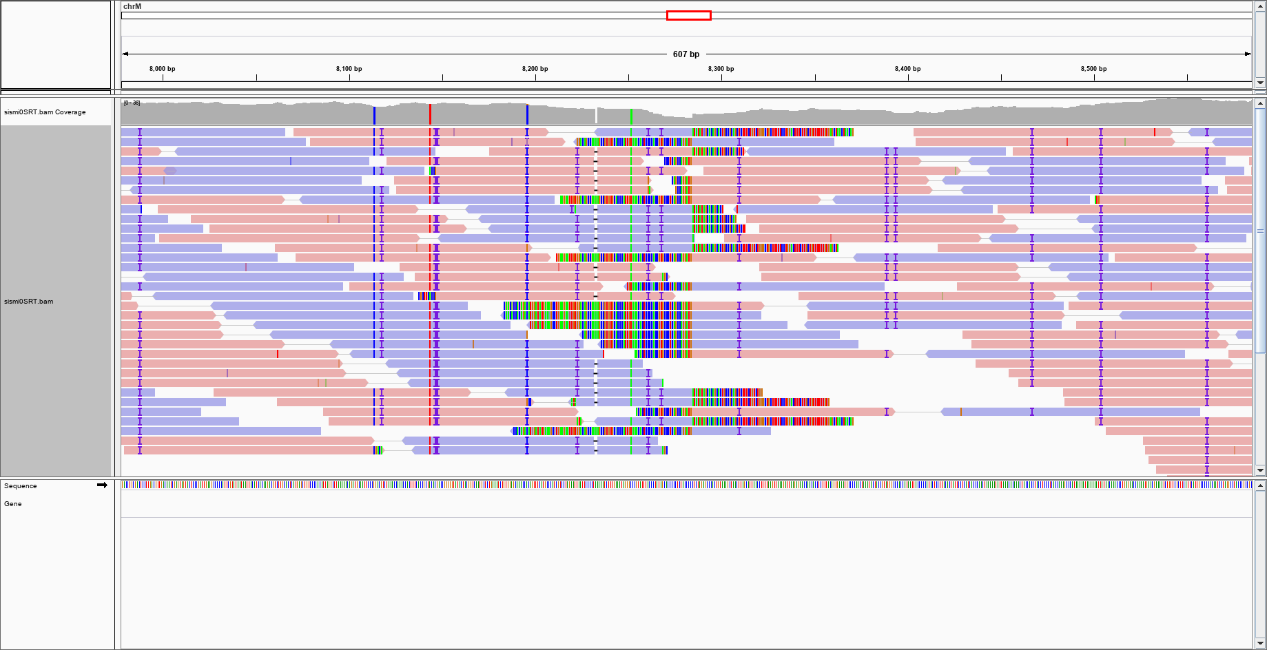
Visualization
- Some tools for visualization and browsing
- IGV (alignments and reference)
- Artemis (genome and annotations)
Visualization
Long reads
Tools for long reads
Take home message
Take home message
→ You have in your hands the first tools to analyze your NGS data
→ Data quality control is a crucial step
→ It is essential to define your plan analyses upstream of your project.
→ NGS are still an ongoing active bioinformatics research field
→ Biostatistics …
References

Module 8bis - Analyse de données NGS sous Galaxy