Analyse de données métagénomiques shotgun
Module 24
March 18, 2024
Introduction
Practical informations
- 9h00 - 17h00
- 2 breaks morning and afternoon
- Lunch at INRAE restaurant (not mandatory)
- Questions allowed
- Everyone has something to learn from each other
Diffusion of documents
All documents presented during this training course are intended for distribution, and are available on https://documents.migale.inrae.fr
Better know you
Who are you?
- Institution / Laboratory / position
What is your scientific topic?
- Studied ecosystem
- Scientific question
- Experimental design
What is your background?
- Already treated shotgun data?
- Background in bioinformatics?
Better know us

- Open infrastructure dedicated to life sciences
- Computing resources, tools, databanks…
- Dissemination of expertise in bioinformatics
- Design and development of applications
- Data analysis
Data analysis service
- We are specialized in genomics/metagenomics
- Bioinformaticians and Statisticians
- More than 120 projects since 2016
- Computational documents used and distributed for reproducibility
- 2 types of services
Collaboration
We take care of the analyses
Accompaniment
We help you to perform the analyses
Training objectives
- Know the advantages and limits of shotgun metagatenomics data analysis
- Identify tools to analyze your data
- Run tools with migale resources
Program
Day 1
- Introduction
- Reminders
- QC
- Taxonomic classification
Day 2
- Cleaning
- Assembly
- Annotation
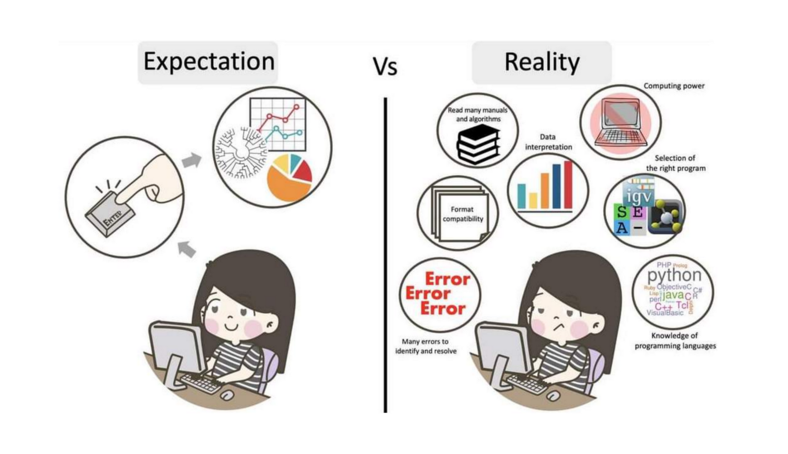
The truth about bioinformatics
Introduction to metagenomics analyses
Introduction
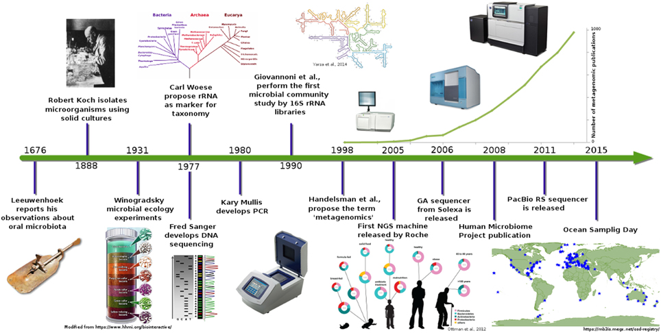
Introduction
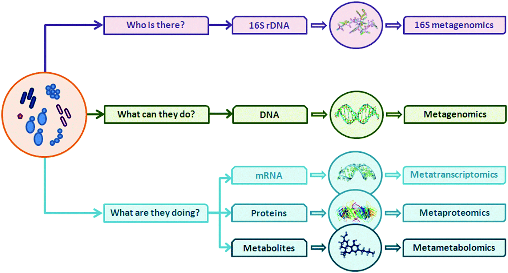
Introduction
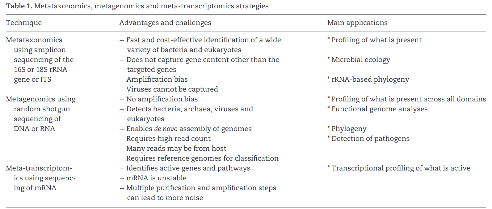
Challenges
- Complexity of the ecosystem
- Completeness of databases
- Sequencing depth
- Computational resources required
- …
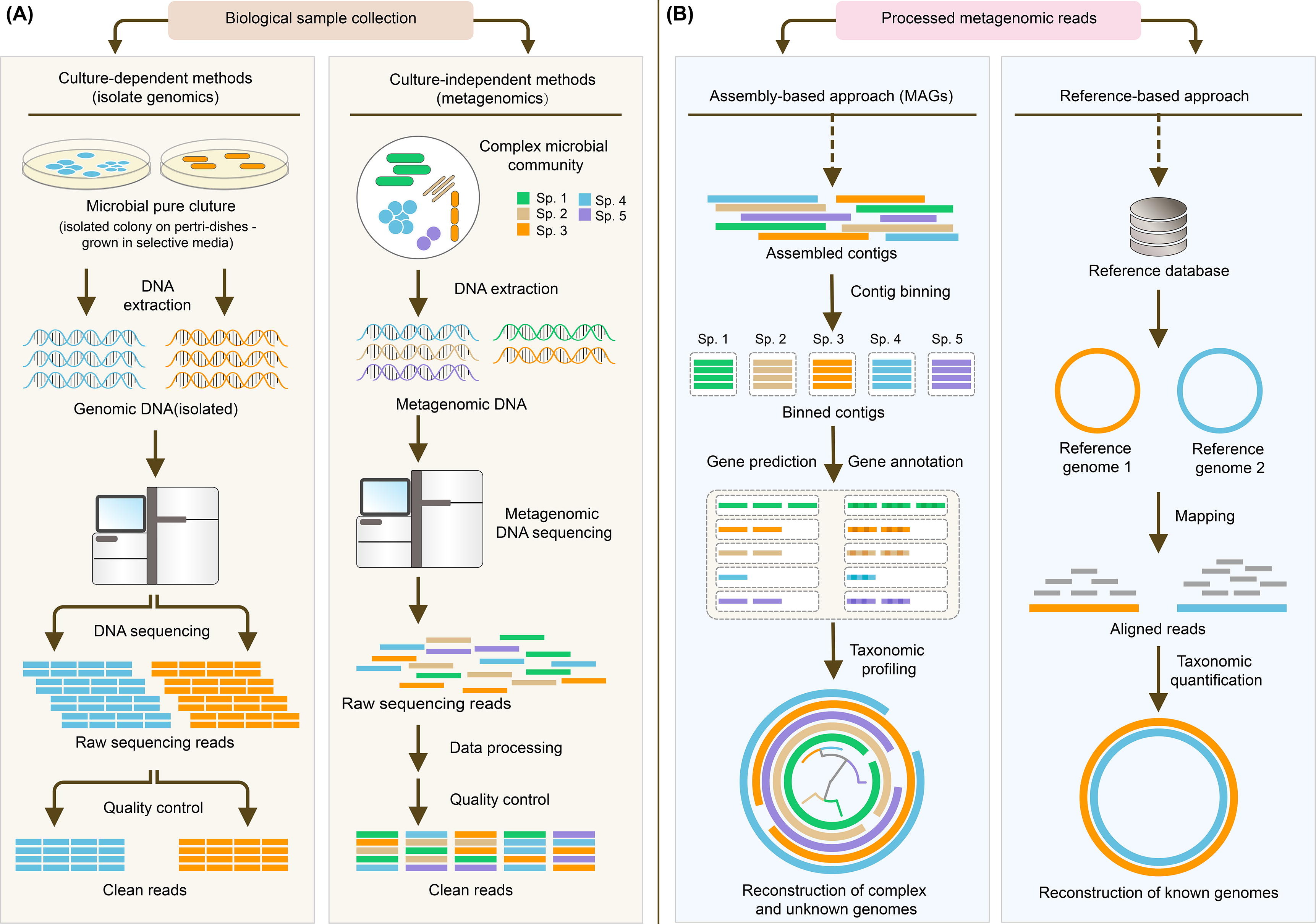
Classical metagenomics approach
Toy datastet presentation
Home-made dataset
- 5 samples
- 1M or 2M reads per sample
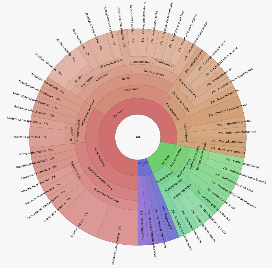
- 50 Bacteria, 10 Archaea, 4 Viruses
- Illumina Hiseq 2x125 bp
- Uniform or log-normal abundance
conda activate insilicoseq-1.5.4
# après un premier tirage aléatoire permettant de récupérer 50 génomes bactériens, 4 génomes viraux et 10 génomes d'archées
iss generate --seed 13062022 -k bacteria viruses archaea -U 50 4 10  --model hiseq --output s1 -n 2000000 --abundance_file hiseq_ncbi_abundance.txt
iss generate --seed 14062022 --genomes s1_genomes.fasta  --model hiseq --output s1 -n 2000000 --abundance_file s1_abundance.txt -z
iss generate --seed 14062022 --genomes s2_genomes.fasta  --model hiseq --output s2 -n 2000000 --abundance_file s2_abundance.txt -z
iss generate --seed 14062022 --genomes s1_genomes.fasta  --model hiseq --abundance uniform --output s3 -n 2000000 -z
iss generate --seed 14062022 --genomes s2_genomes.fasta  --model hiseq --abundance uniform --output s4 -n 1000000 -z
iss generate --seed 14062022 --genomes s1_genomes.fasta  --model hiseq --output s5 -n 2000000 --abundance_file s1_abundance.txt -z
Dataset composition
Reminders about command line
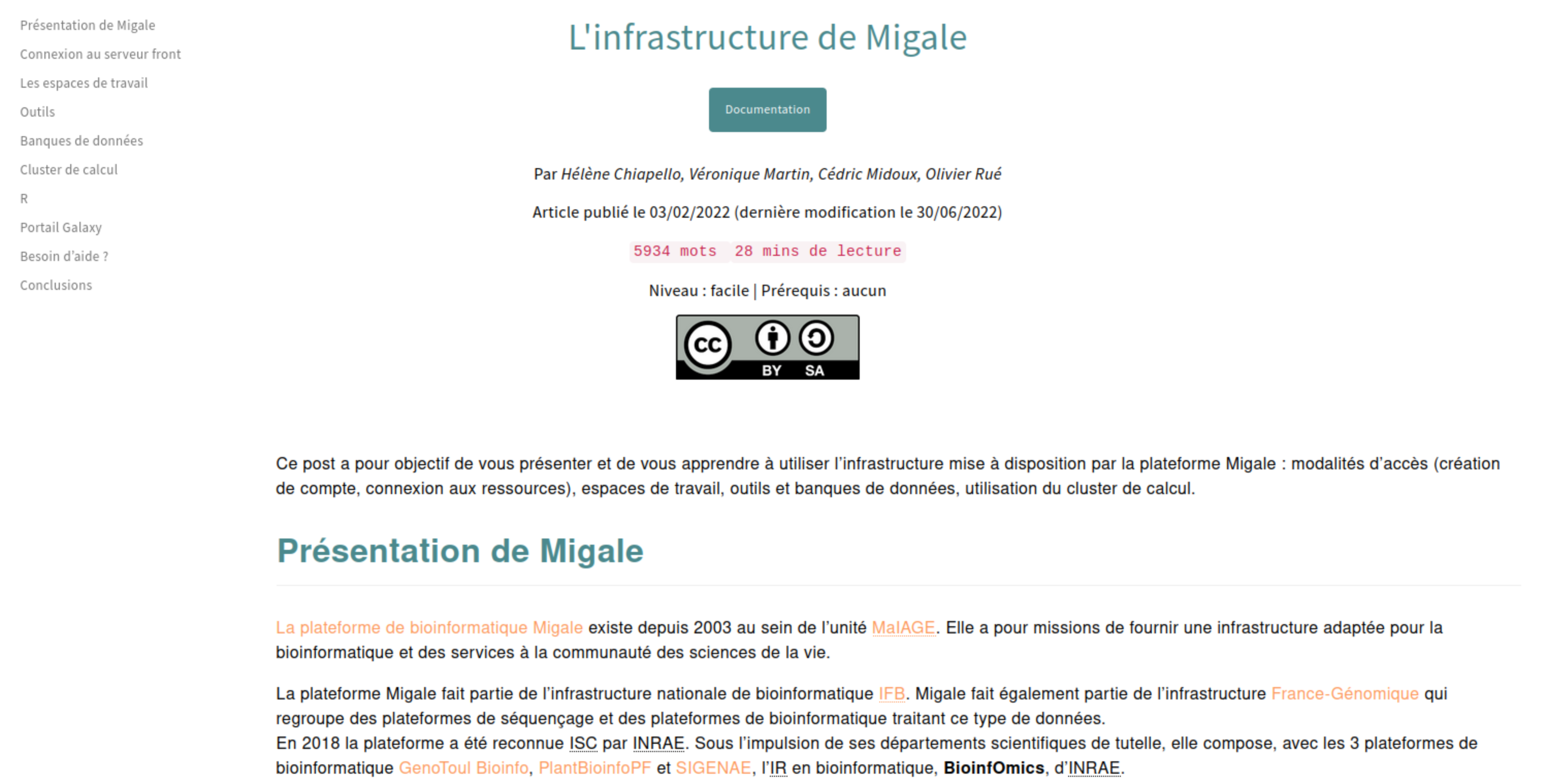
The migale facility
- working directories (
save/work/home) - SGE submission system (
qsub/qstat) - conda environments (
conda activate)
All usefull information
Switch to TP 1
Reminders about sequencing
Generations
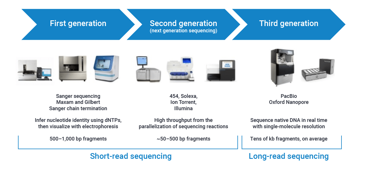
We will only deal with short reads during this training
Reminders about Illumina sequencing
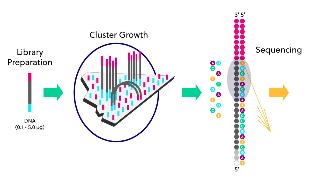
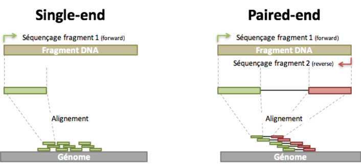
Sequencing - Vocabulary
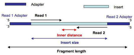
- Read: piece of sequenced DNA
- DNA fragment: 1 or more reads depending on whether the sequencing is single- or paired-end
- Insert: Fragment size
- Depth: \(\frac{N * L}{G}\)
\(N =\) number of reads
\(L =\) reads size
\(G =\) genome size - Coverage: % of genome covered

FASTQ format
Meaning
@Identifier1 (comment)
XXXXXXXXXXXXXXXXXXXXXXXXXXXXXXXXXXXXXXXXXXXXXXXXXXXXXXX
+
QQQQQQQQQQQQQQQQQQQQQQQQQQQQQQQQQQQQQQQQQQQQQQQQQQQQQQQ
@Identifier2 (comment)
XXXXXXXXXXXXXXXXXXXXXXXXXXXXXXXXXXXXXXXXXXXXXXXXXXXXXXXXXXXXXXXXXX
+
QQQQQQQQQQQQQQQQQQQQQQQQQQQQQQQQQQQQQQQQQQQQQQQQQQQQQQQQQQQQQQQQQQ
Quality score encoding

Quality score
Measure of the quality of the identification of the nucleobases generated by automated DNA sequencing

FASTQ compression
- Compression is essential to deal with FASTQ files (reduce disk storage)
- extension:
file.fastq.gz - Tools are (almost all) able to deal with compressed files
Quality control
Quality control
- One of the most easy step in bioinformatics …
- … but one of the most important
- check if everything is ok
- Indicates if/how to clean reads
- Shows possible sequencing problems
- The results must be interpreted in relation to what has been sequenced
Reads are not perfect

Why QC’ing your reads?
Try to answer to (not always) simple questions:
- Are data conform to the expected level of performance?
- Size / Number of reads / Quality
- Residual presence of adapters or indexes?
- (Un)expected techincal biases?
- (Un)expected biological biases?
Using callouts is an effective way to highlight content that your reader give special consideration or attention.
Switch to TP 2
Taxonomic affiliation
Taxonomic affiliation
Definition
Taxonomic assignment in the context of bioinformatics involves the computational identification and classification of organisms into their taxonomic groups using various data sources, such as DNA sequences, protein sequences, or other molecular markers. This process typically utilizes algorithms and computational tools to compare sequences against reference databases or phylogenetic trees, allowing for accurate identification and classification of organisms at different taxonomic levels.

Kraken
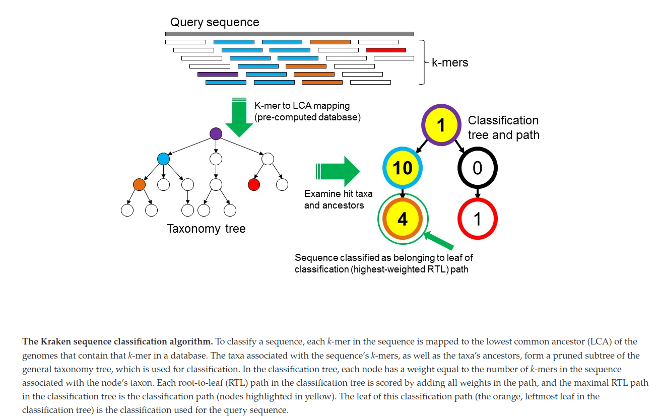
Kraken [5] is a very popular taxonomic affiliation tool. It is very fast and accurate. Kraken examines the k-mers (~35 bp) within the query sequence, searches for them in the database, looks for where these are placed within the taxonomy tree inside the database, makes the classification with the most probable position, then maps k-mers to the lowest common ancestor (LCA) of all genomes known to contain the given k-mer.
Method:
- Chop genomes into k-mers and link to a taxonomic id.
- Chop reads into k-mers and search for exact hits in database
- Search for highest-wighted root-to-leaf paths and assign the taxonomic id of the lowest node to read
Kraken
Kaiju
Kaiju [6] is an equivalent of Kraken, but with some particularities:
- Database of proteic sequences
- Supposed to be more sensitive
- Translate reads in all six reading frames, split at stop codons
- Use BWT and FM-index table
Kaiju databanks
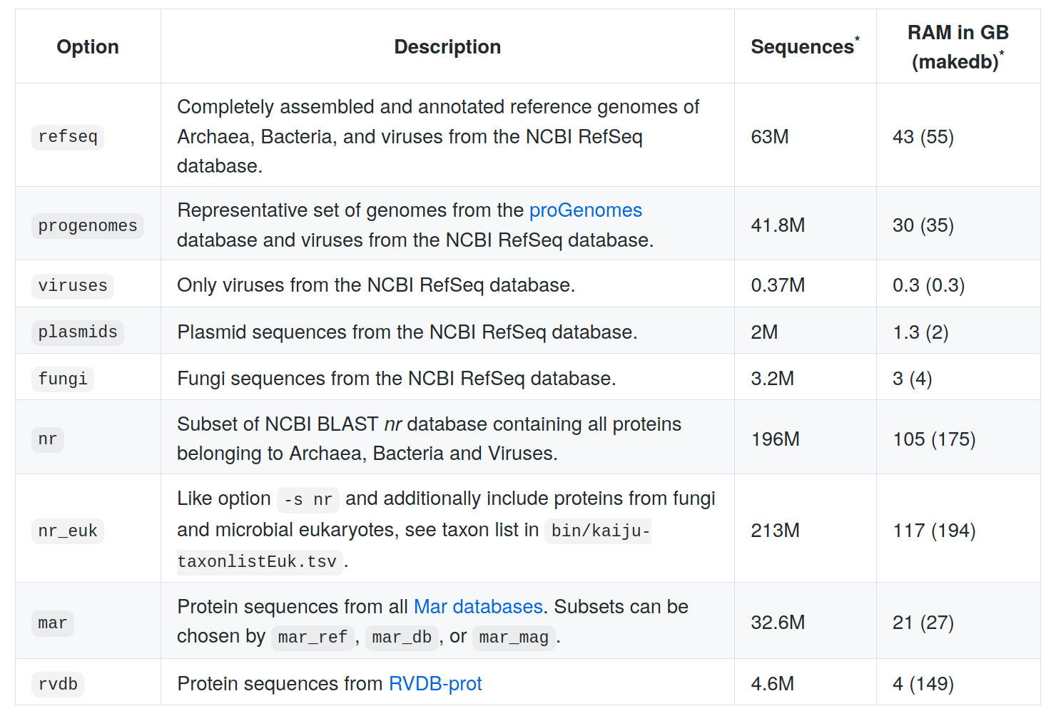
Taxonomic classification caveats
- Databanks
- K-mer choice (sensitivity / specificity)
- Allow a “fast” overview of your data
- Contaminants?
- Host reads?
- Classification rate
Some taxonomic affiliation tools
| tool | migale | comments |
|---|---|---|
| Kraken2 | ✔️ | the reference, fast and efficient |
| Kaiju | ✔️ | protein level |
| Bracken | ✔️ | Bayesian Reestimation of Abundance with Kraken |
| Centrifuge | ✔️ | indexing scheme based on the Burrows-Wheeler transform (BWT) and the Ferragina-Manzini (FM) index, optimized specifically for the metagenomic classification problem |
| MetaPhlAn3 | ✔️ | MetaPhlAn relies on unique clade-specific marker genes identified from ~17,000 reference genomes (~13,500 bacterial and archaeal, ~3,500 viral, and ~110 eukaryotic) |
Switch to TP 3
Reads cleaning
Quality/Length/Adapters
- Detect and remove sequencing adapters present in the FASTQ files
- Filter / trim reads according to quality (seen with FastQC)
rRNA removal
- Mandatory step if you want to skip rRNA reads
Contamination
Definition
Contamination corresponds to the presence of DNA that does not come from the sample studied.
- Recognizing contamination, followed by appropriate decontamination, should be a critical first step for all microbiome analyses.
- Skipping this step can easily result in confounded results and false conclusions.
Contamination origins
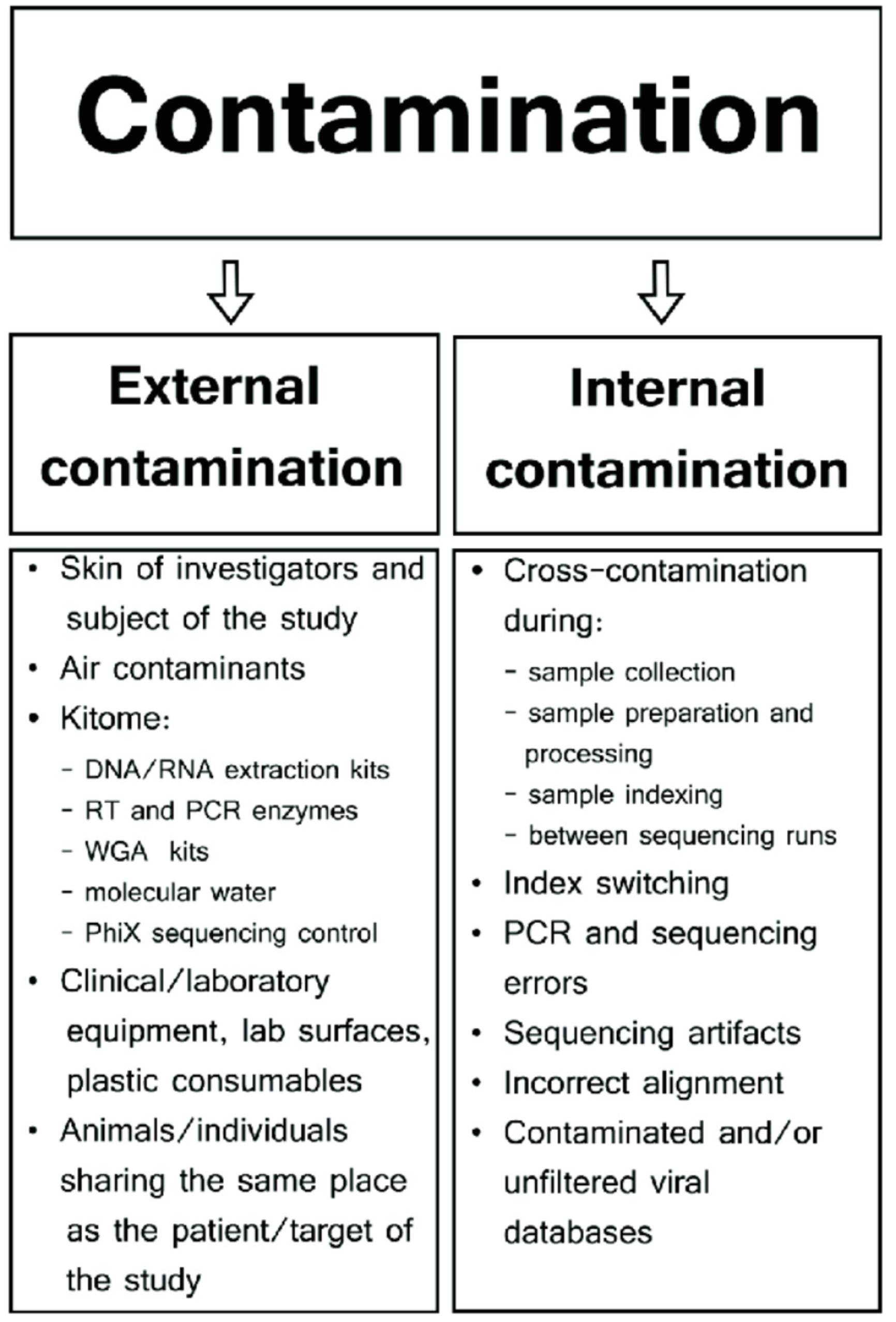
External contaminants
- negative controls (i.e., blank reagent controls) during sample collection, preparation, and/or sequencing
- in silico detection (taxonomic affiliation, mapping…)
Well-to-well contamination
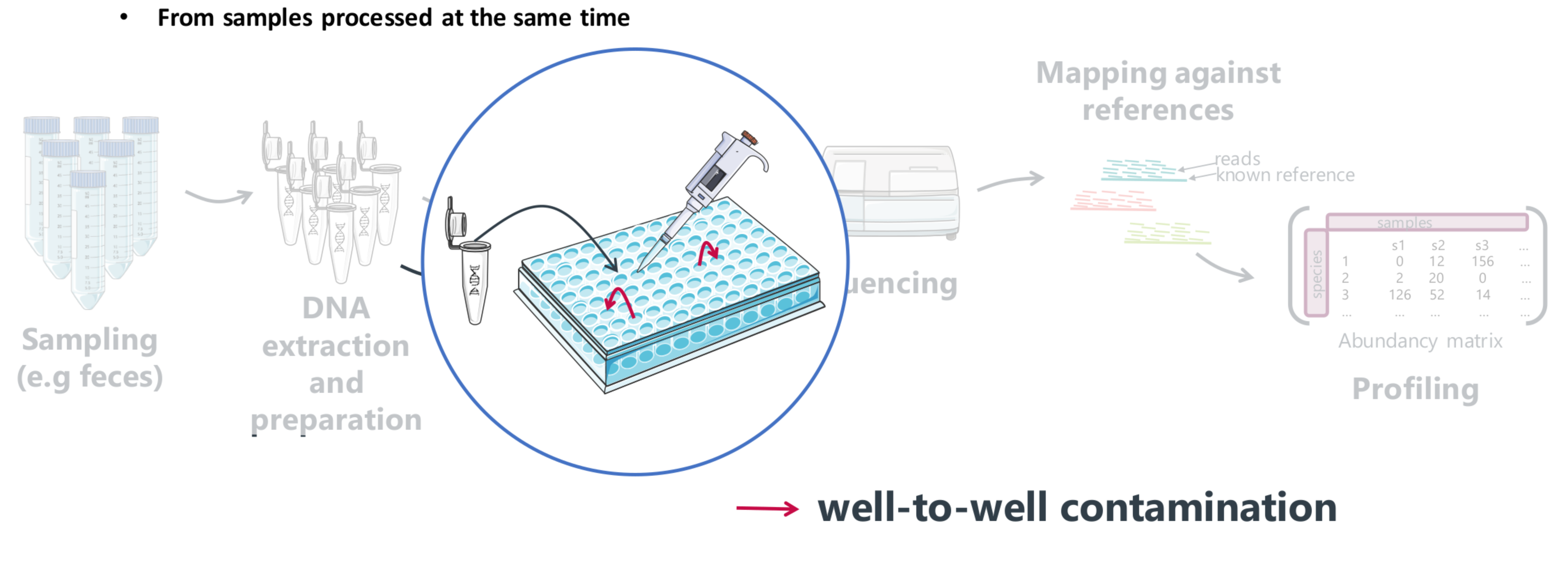
Cleaning tools
Reads cleaning
| tool | migale | comments |
|---|---|---|
| fastp [10] | ✔️ | all in one |
| pear [11] | ✔️ | for merging reads |
| sickle [12] | ✔️ | adaptative trimming |
Decontamination tools
| tool | migale | comments |
|---|---|---|
| kneaddata [13] | ✔️ | remove rRNA reads |
| sortmerna [14] | ✔️ | remove rRNA reads, slow… |
| HoCoRT [15] | ✔️ | choice between several aligners, easy to use |
| DeconSeq | ❌ | |
| GenCoF | ❌ |
Switch to TP 4
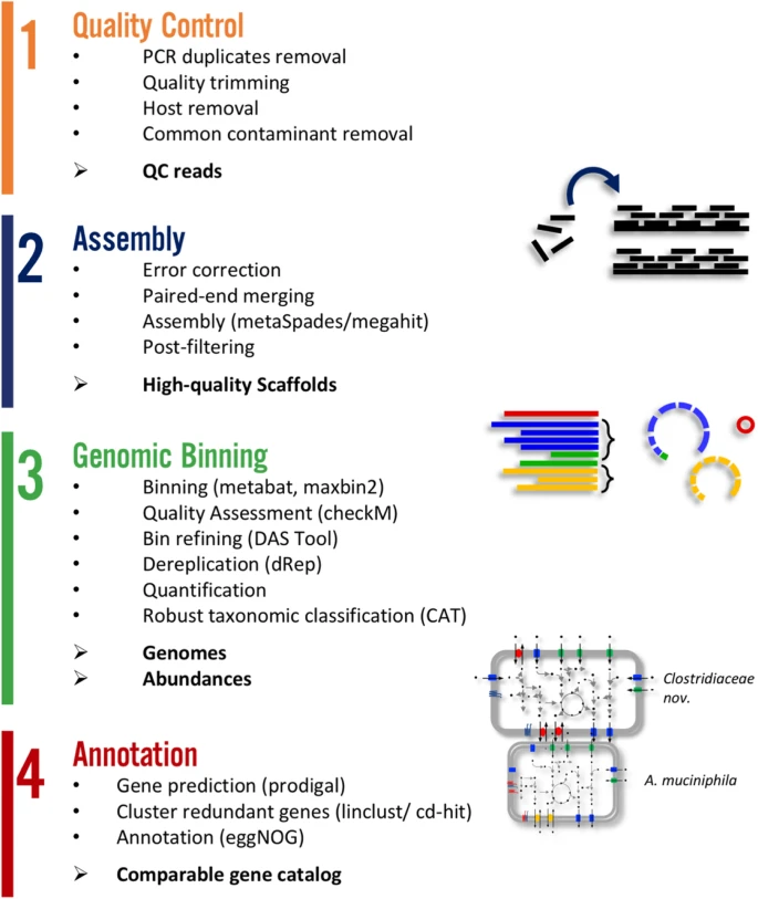
Metagenomics assembly
Objectives
- Reconstruct genes and organisms from complex mixtures
- Dealing with the ecosystem’s heterogeneity, multiple genomes at varying levels of abundance
- Limiting the reconstruction of chimeras
Assembly strategies
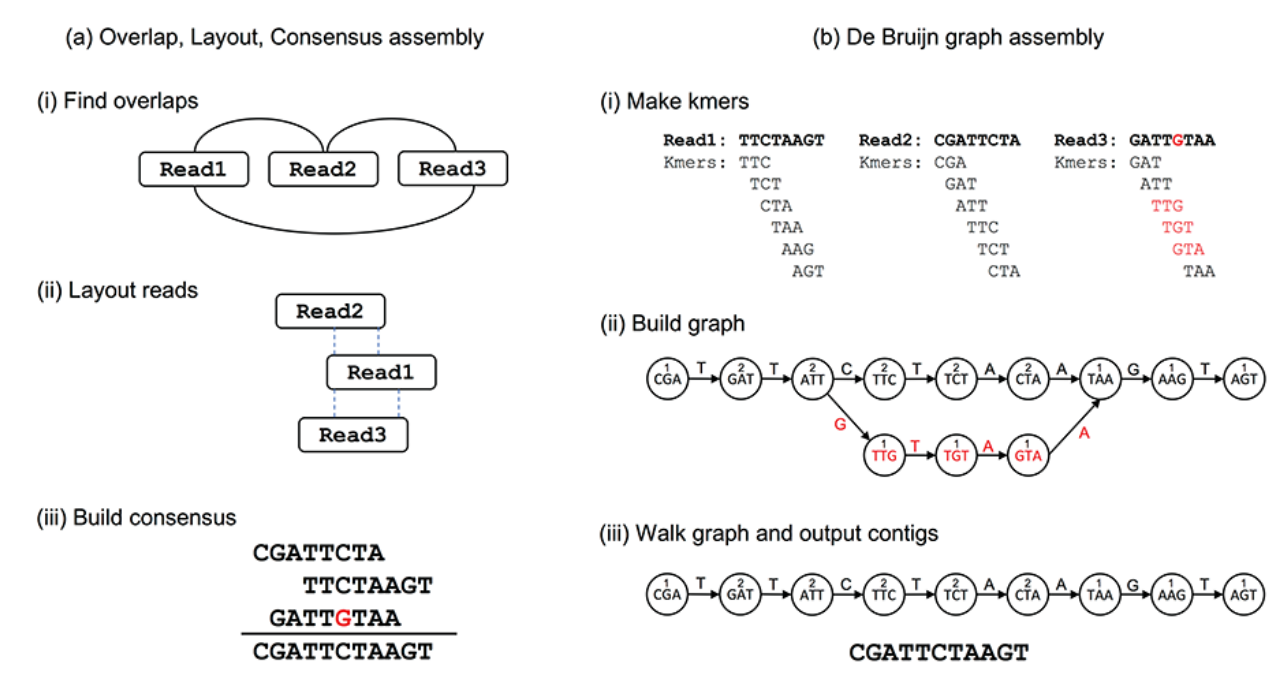
Co-assembly?
- Usefull in some cases:
- differences in coverage between samples
| Pros of co-assembly | Cons of co-assembly |
|---|---|
| More data | Higher computational overhead |
| Better/longer assemblies | Risk of shattering the assembly |
| Access to lower abundant organisms | Risk of increased contamination |
Co-assembly
In these cases, co-assembly is reasonable if:
- Same samples
- Same sampling event
- Longitudinal sampling of the same site
- Related samples
If it is not the case, individual assembly should be prefered. In this case, an extra step of de-replication should be used
Tools
- Generic tool with a meta option : SPAdes and metaSPAdes [16]
- Tools requiring less memory : MEGAHIT [17]
- The historical tool allowing many parameters : Velvet (and MetaVelvet)
- A (not so) recent benchmark of short reads metagenome assemblers. [18]
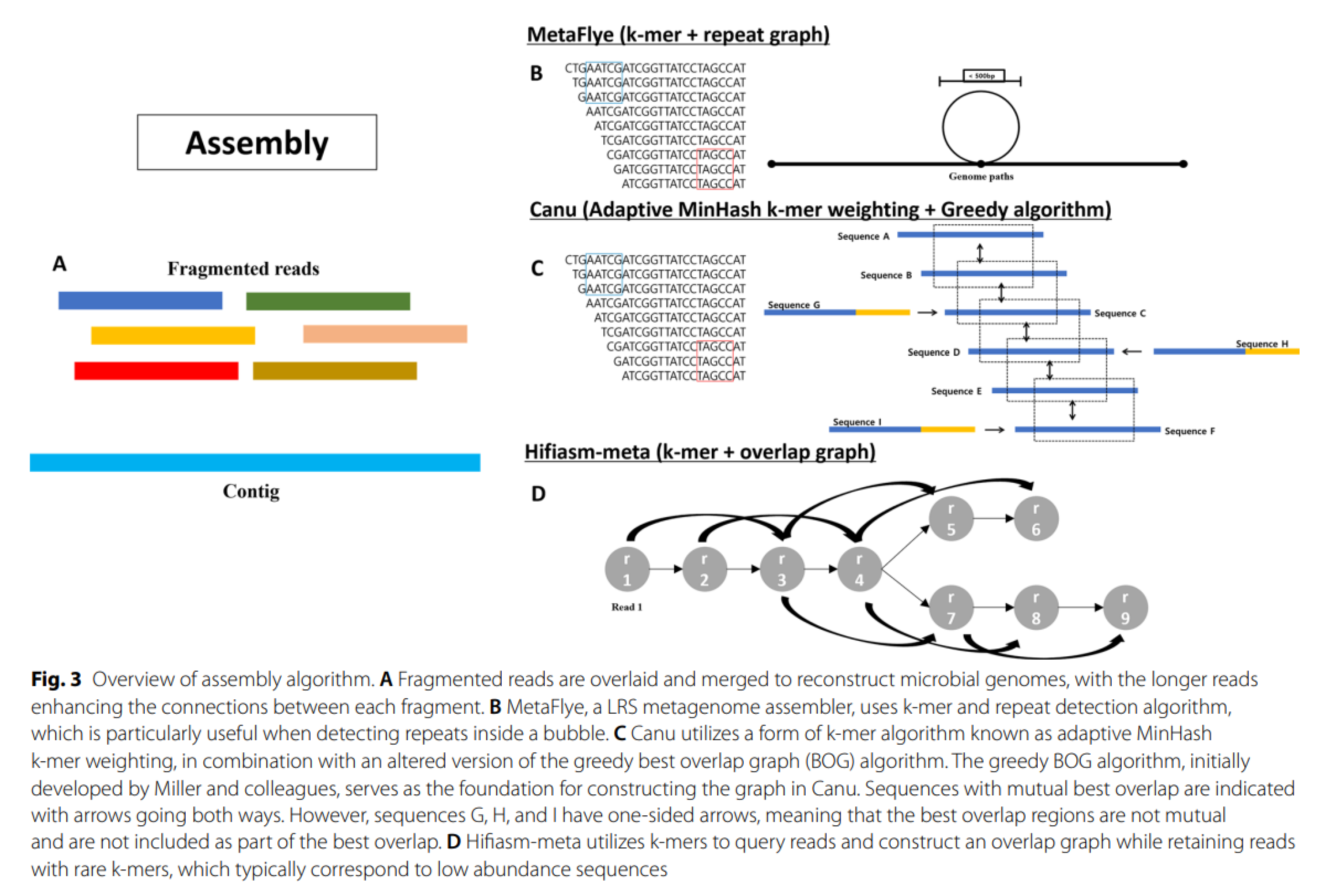
- Long read / Hybrid assemblies use different algorithms and strategies and are still a research question.
Assessment of assembly quality
After assembly, we use MetaQUAST [19] to evaluate and compare metagenome assemblies.
What MetaQUAST does :
- De novo metagenomic assembly evaluation
- [Optionally] identify reference genomes from the content of the assembly
- Reference-based evaluation
- Filtering so-called misassemblies based on read mapping
- Report and visulaisation
De novo metrics
Evaluation of the assembly based on:
- Number of contigs greater than a given threshold (0, 1kb, …)
- Total / thresholded assembly size
- Largest contig size
- N50 : the sequence length of the shortest contig at 50% of the total assembly length, equivalent to a median of contig lengths. (N75 idem, for 75%)
- L50 : the number of contigs at 50% of the total assembly length. (L75 idem, for 75%)
Reference-based metrics
- Metrics based on the comparison with reference genomes.
- Reference genomes are given by the user or automatically constitued by MetaQuast based on comparison of rRNA genes content of the assembly and a reference database (Silva).
- Complete genomes are then automatically downloaded.
Reference-based metrics
For each given reference genome, based on an alignement of all contigs on it :
- Duplication rate
- Percent genome complete
- NGA50 : equivalent of N50 but with the aligned block of the contigs
- “Misassemblies” : breakpoint of alignement in a contigs.
- An individual Quast report and an alignement visualisation.
Counts on assembly
- We used only a portion of the reads for assembly.
- For further analyses it is necessary to map all the reads on the contigs to obtain counts per features (genes/contigs…)
- We will use BWA [20]
Switch to TP 5
Binning
Objectives
Binning is a good compromise when the assembly of whole genomes is not feasible.
Similar contigs are grouped together.
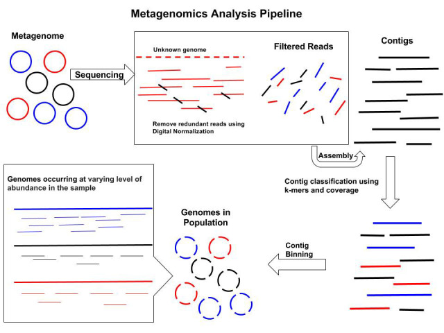
Approach
- MetaBAT [23] is a tool for reconstructing genomes from complex microbial communities.
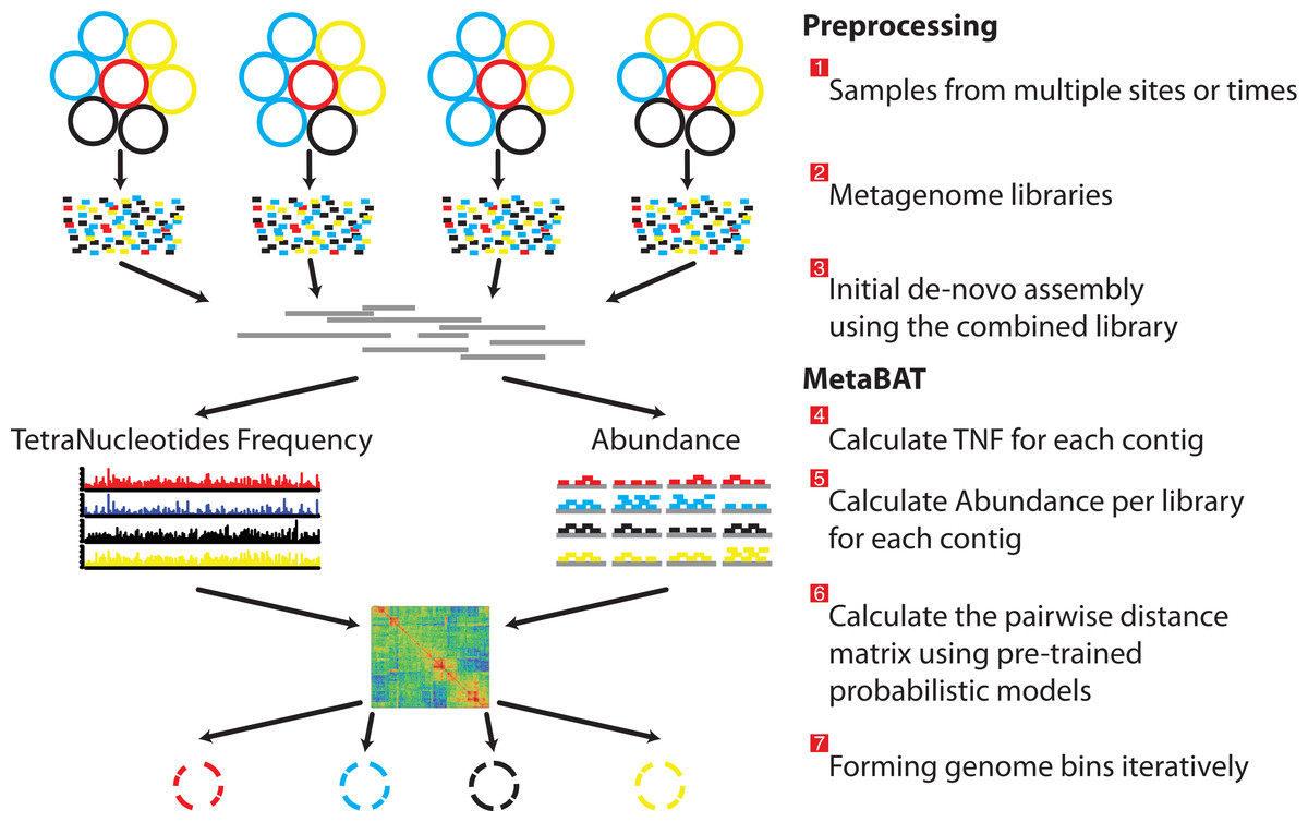
Bins evaluation
For the evaluation of bins, we will use completeness and contamination estimated by CheckM [24]
- Use of collocated sets of genes that are ubiquitous and single-copy within a phylogenetic lineage.
- Among a set of tools in CheckM we will use the
checkm2 predictworkflow which only mandatory requires a directory of genome bins.
Switch to TP 6
Annotation
Objective
- Syntaxic annotation (gene prediction)
- Functionnal annotation (function prediction for protein coding genes)
- Prokka [25] is a is a software tool to annotate bacterial, archaeal and viral genomes (quite) quickly and produce standards-compliant output files.
- Prokka automatically annotate a complete bacterial genome in ~15mn.
- Prokka will not replace expert annotation but gives you an homogenoeus procedure for annotation of conserved genes familly
Genes prediction (1)
- Gene prediction in complete prokaryotic genomes isn’t as such a problem.
- Most errors / difference in start position
- Efficient gene predictors are available (bactgeneSHOW, prodigal, glimmerHMM,…).
- Most of them uses HMM (Hidden Markov Models) models to predict the gene structure
Genes prediction (2)
- Gene prediction on metagenomes is difficult due to :
- assembly fragmentation
- assembly errors, frameshift, chimeras,…
- different species in the same sample that could/should lead to use different models
- a mix of viral, bacterial and eukaryotic sequences.
- Prodigal (with the
-metaparameter) and fraggenescan have good enough results on metagenomic contigs. - Caution to partial genes in the following analysis !
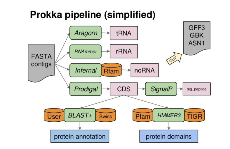
Prokka pipeline
- Coding gene prediction with Prodigal [26]
- tRna; rRna gene prediction with Aragorn, Barnap, RNAmmer (optionnal)
- Functionnal annotation based on similarity search with a threshold (1e-6) and hierarchically against :
- [Optionnal] a given proteome (
--proteinsparameter) - ISFinder for transposases, not entire IS
- NCBI Bacterial Antimicrobial Resistance Reference Gene Database for Antimicrobial Resistance Genes.
- UniprotKB/Swissprot curated proteins with evidence that (i) from Bacteria (or Archaea or Viruses); (ii) not be “Fragment” entries; and (iii) have an evidence level (“PE”) of 2 or lower, which corresponds to experimental mRNA or proteomics evidence.
- Domain and motifs (hmmsearch) :
- [Optionnal] a given proteome (
Prokka pipeline
EggNogg Mapper
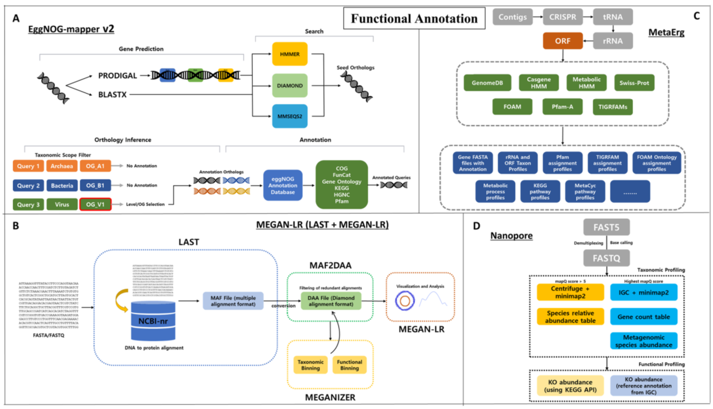
- eggNOG-mapper [27] is a tool for fast functional annotation of novel sequences. It uses precomputed orthologous groups and phylogenies from the eggNOG database to transfer functional information from fine-grained orthologs only.
- eggNog database :
- 5090 organisms, 2502 viruses.
- 4.4 M orthologous groups annotated with COG category, Gene Ontolgy, EC number, Kegg orthologs and pathways, CAZy, PFAMs
EggNogg Mapper workflow
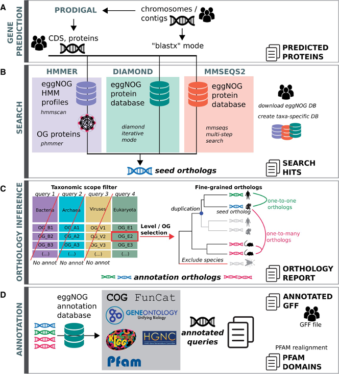
- eggNOG uses hmmsearch to search against HMM eggNOG database OR Diamond / MMSeqs2 to search against eggNOG protein database
- Refine first hit using a list of precomputed orthologs.
- Assign one ortholog
- Functionnal annotation transfer using this ortholog
Other options for functionnal annotation
- Diamond [28] is a sequence aligner for protein (equivalent blastp) and translated DNA (equivalent tblastx) searches, designed for high performance analysis of big sequence data. Diamond is 100x to 20,000x the speed of BLAST.
- Diamond could be used to query against any given databank.
- ghostKOALA [29, Online]
- KOALA (KEGG Orthology And Links Annotation) is KEGG’s internal annotation tool for K number assignment.
Other options for functionnal annotation (2)
- cd-hit [30] is a software for clustering protein sequences. It can be used to downsize the number of lines in the in the gene count matrix.
Switch to TP 7
Biostatistics
What to do after bioinformatics
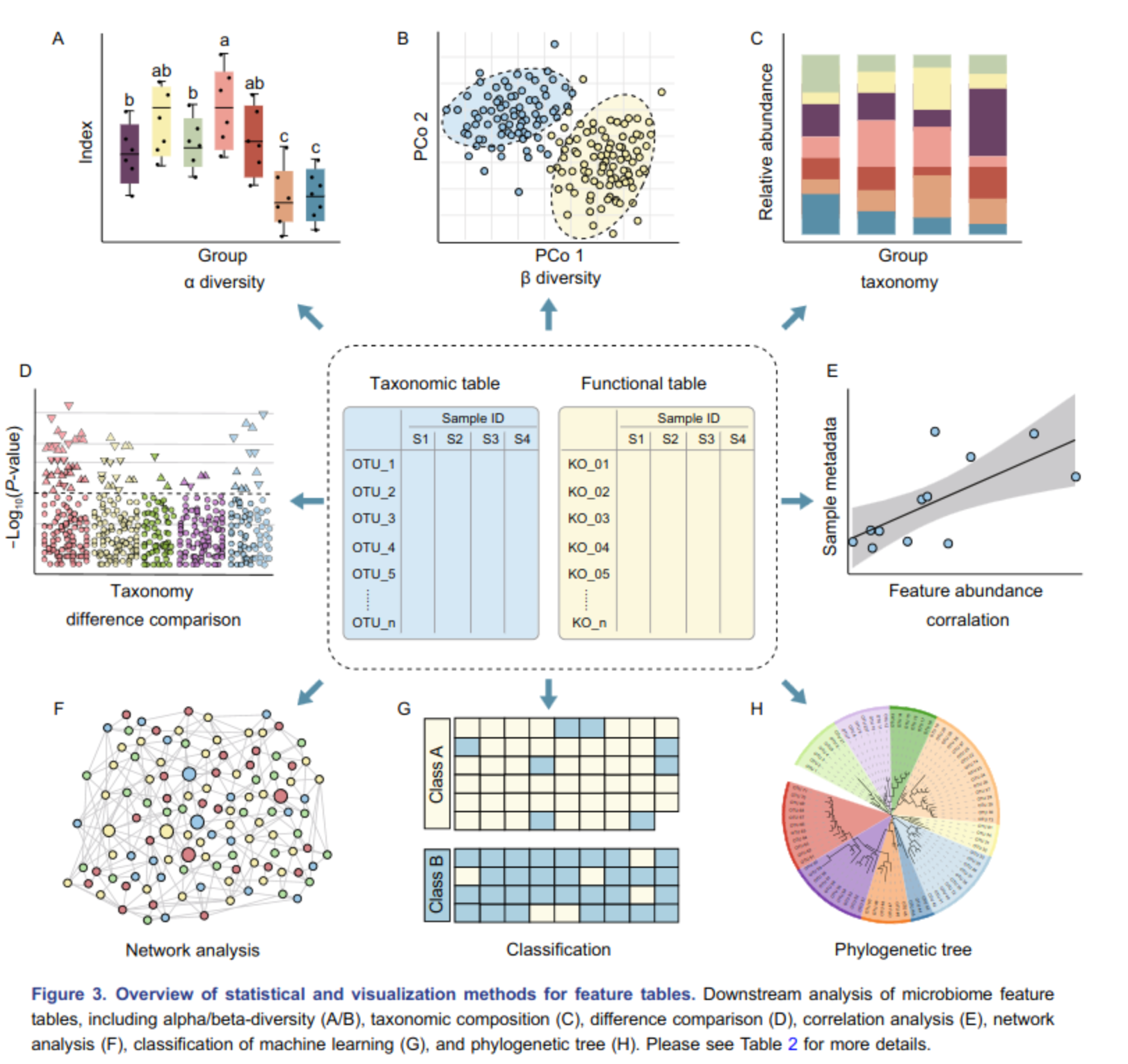
Automatization
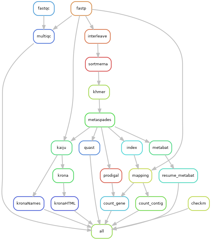
Snakemake workflow
We have developed a workflow that allows us to automate all these analyses.
- developed with snakemake
- executable on MIGALE
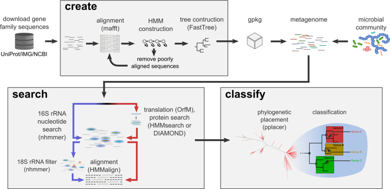
Other tools
GraftM: rapid community profiles from metagenomes
Anvi’o: integrated multi-omics at scale
- Anvi’o [35] is an open-source, community-driven analysis and visualization platform for microbial ’omics.
- With this tutorial, starting from a metagenomic assembly, you will :
- Process your contigs,
- Profile your metagenomic samples and merge them,
- Visualize your data, identify and/or refine genome bins interactively, and create summaries of your results.
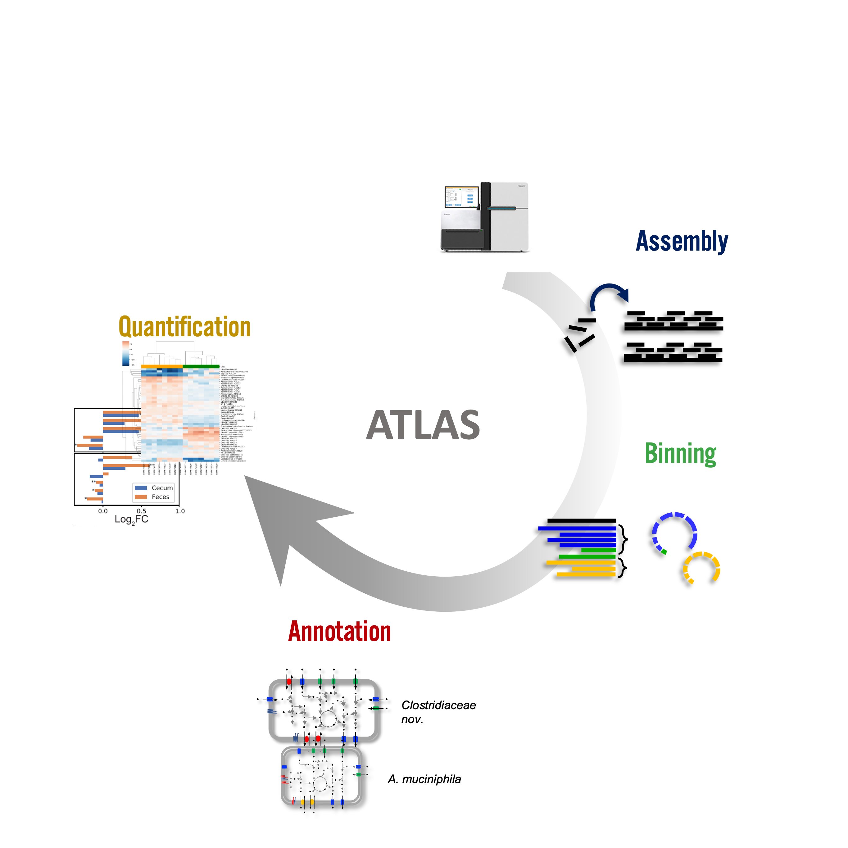
Metagenome atlas
- Metagenome-atlas [36] is an easy-to-use metagenomic pipeline based on
snakemake. - It handles all steps of analysis :
Metagenome atlas
Long reads metagenomics

Long reads metagenomics
Long reads metagenomics
Taxonomic classifiers

Long reads metagenomics
Functional annotation
Long reads metagenomics
- Long read data can be used to improve assembly
- Bottlenecks :
- DNA extraction (?)
- cost of data generation
- sequencing errors
- State of the art pipeline for assembly :
- standalone long read assembly (ex: MetaFLYE [38])
- optional error correction with short reads
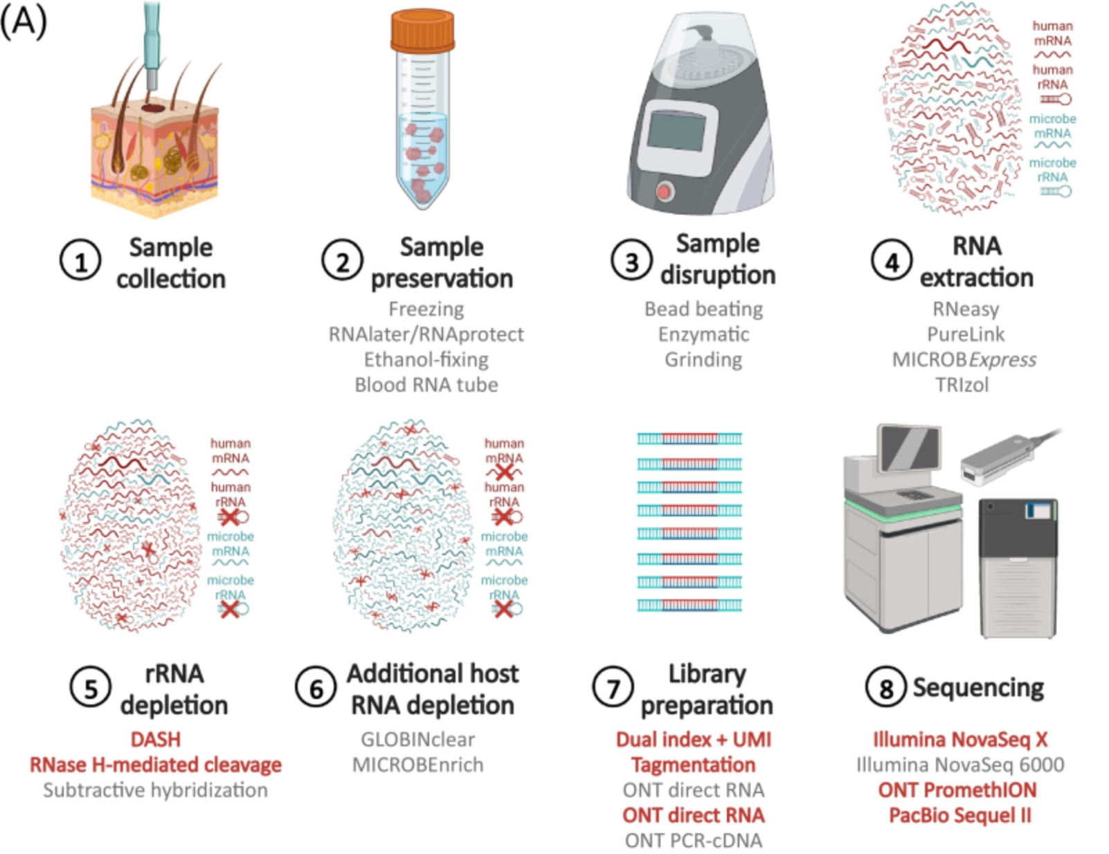
Metatranscriptomics
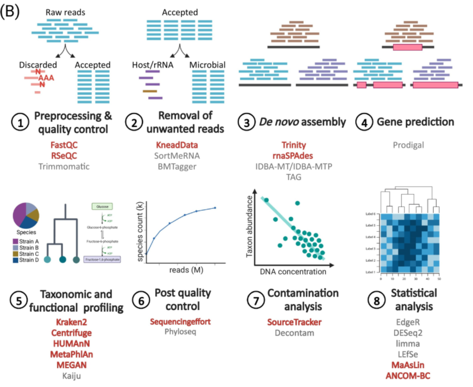
- Shotgun metagenomics is still an ongoing active bioinformatics research field
- Numerous software dedicated to assembly, binning, functional annotation are actively developed
- Depending on the ecosystem , one can have different approaches :
- mapping on a reference database
- assembly and mapping
- The biological question must determine the analysis
- Any question at help-migale@inrae.fr
- Need tool? https://migale.inrae.fr/ask-tool
- Need more resources? https://migale.inrae.fr/ask-resources
- Need more help than just one question? https://migale.inrae.fr/ask-data-analysis
References

Module 24 - Métagénomique shotgun