Microbiome biodiversity
Some slides were adapted from Mahendra Mariadassou’s supports
Different type of diversity indices
- \(\alpha\)-diversity: diversity within a sample/community
- which community is more diverse ?
- \(\beta\)-diversity: diversity between samples/communities
- Which communities are most similar?
- \(\gamma\)-diversity: total species diversity across a landscape, combining local \(\alpha\)-diversity and \(\beta\)-diversity differences among sites
\(\alpha\)-diversity
How many species in each sample/community ? Distribution of species ?
- quantitative measure of the biodiversity within a sample/community
- at the ASV level or any other taxonomic rank
4 categories, the most popular indices
- Richness: Observed, Chao1
- Information (Abundance distribution): Shannon
- Dominance (or Evenness): Simpson, invSimpson
- Phylogenetics: Faith
\(\alpha\)-diversity - Richness based
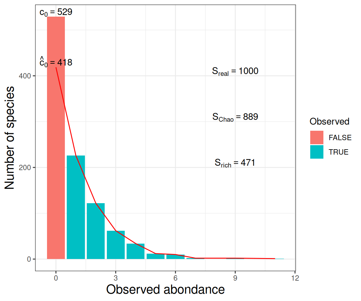
- Number of observed species
- \(\text{Observed} = \sum_{s} 1_{\{p_s > 0\}} = \sum_{i} c_i = \text{S}\)
- Observed + (estimated) number of unobserved species
- \(\text{Chao1} = \text{Observed} + \hat{c}_0\)
Note \(c_i\) the number of species observed \(i\) times (\(i = 1, 2, \dots\)) and \(p_s\) the proportion of species \(s\) (\(s = 1, \dots, S\)).
\(\alpha\)-diversity - Shannon
- Shannon
- \(\text{H} = - \sum_{s} p_s \log\left( p_s \right)\)
Note \(p_s = n_{s}/N\) the proportion of species \(s\) (\(s = 1, \dots, S\)), \(n_{s}\) number of species \(s\) et \(N\) total number of species.
Take into account the relative abundance of each taxon \(p_s\)
- H = 0 when the sample contains only one specie.
- H increases when the number of different species increases. In other words, the diversity is high.
- H = log(S) is maximal when each species is equally representated.
\(\alpha\)-diversity - Eveness
- Simpson diversity (D)
- \(\text{D} = p_1^2 + \dots + p_S^2\)
- inverse Simpson, inverse probability that two sequences sampled at random come from the same species
- \(\text{InvSimpson} = \frac{1}{p_1^2 + \dots + p_S^2} \leq S\)
Take into account the relative abundance of each taxon \(p_s\)
Capture how dominated a community is by its most abundant taxa, asking “What is the probability that two randomly chosen sequences belong to the same taxon?”
Interpretation: - If one specie dominates completely : D = 1 and 1/D = 1 (minimal value) - 1/D increases with diversity (as would Shannon, richness and others)
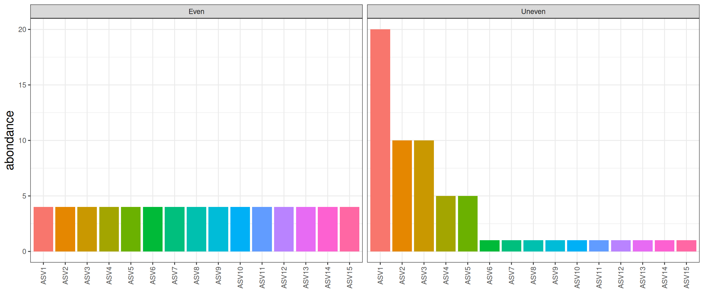
\(\alpha\)-diversity - illustration
| Observed |
15 |
15 |
| Shannon |
2.71 |
2.06 |
| invSimpson |
15 |
5.45 |
Low Shannon and invSimpson, communities are dominated by a few abundant taxa.
\(\alpha\)-diversity - filtering
Many \(\alpha\) diversities (Observed, Chao) depend a lot on rare ASV. Do not trim rare ASV before computing them as it can drastically alter the result.
Practice
Consider working with rarefied data
- Produce \(\alpha\) diversity table
- Explore \(\alpha\) diversities
\(\alpha\) diversity - Test (1/2)
Perform an analysis of variance (ANOVA) to test the impact of some covariates in the experimental design (in the sample_data table).
Test the null hypothesis \(H_O\), there is no difference between the biological conditions (groups) versus the mean is different between groups.
Assumptions
- \(\epsilon \sim_{iid} \mathcal{N}(0,\,\sigma^{2})\)
- Gauss law, independence, heteroscedasticity
\(\alpha\) diversity - Test (2/2)
Reject \(H_0\) when \(Pr(F > f) \leq \alpha\) (significant level, 5% usually)
To understand group differences in ANOVA, conduct post hoc tests also called “multiple comparison analysis” tests.
- Easy16S: Tukey’s Honest Significant Differences
Practice
Test and interpret
- The seasonal effect on \(\alpha\) diversity
- The AOP effect on \(\alpha\) diversity
- The seasonal effect on \(\alpha\) diversity inside a fixed AOP (subset)
\(\alpha\) diversity - rarefaction
best approach to control for uneven sequencing effort
Schloss PD. 2024. Rarefaction is currently the best approach to control for uneven sequencing effort in amplicon sequence analyses. mSphere 9:e00354-23. https://doi.org/10.1128/msphere.00354-23
\(\beta\) diversity
- \(\beta\)-diversity: diversity between samples/communities
- Which communities are most similar/dissimilar accross samples?
Jaccard index
measures the fraction of species specific to either A or B
\({\text{Jaccard}} = \frac{\sum_{s} 1_{\{n^A_s > 0, n^B_s = 0 \}} + 1_{\{n^B_s > 0, n^A_s = 0 \}}}{\sum_{s} 1_{\{n^A_s + n^B_s > 0 \}}}\)
Note \(n^A_s\) the count of species \(s\) (\(s = 1, \dots, S\)) in community \(A\) and \(n^B_s\) the count in community \(B\). We focus on shared taxa.
A simple example
| 🌹 |
50 |
10 |
| 🌻 |
10 |
50 |
| 🌸 |
20 |
5 |
| 🌼 |
5 |
20 |
| Total |
85 |
85 |
Result:
\[
\frac{0}{4 + 4} = 0
\]
Jaccard index
measures the fraction of species specific to either A or B
\({\text{Jaccard}} = \frac{\sum_{s} 1_{\{n^A_s > 0, n^B_s = 0 \}} + 1_{\{n^B_s > 0, n^A_s = 0 \}}}{\sum_{s} 1_{\{n^A_s + n^B_s > 0 \}}}\)
Note \(n^A_s\) the count of species \(s\) (\(s = 1, \dots, S\)) in community \(A\) and \(n^B_s\) the count in community \(B\).
Focus on shared taxa.
- Jaccard = 0 when all taxa are shared
- Jaccard = 1 when all taxa are specific
Bray Curtis distance
The Bray Curtis distance mixes which species are present in each sample and how abundant they are.
\(\displaystyle {\text{BC}} = \sum_{s} |n^A_s - n^B_s| / \sum_{s} |n^A_s + n^B_s|\)
Note \(n^A_s\) the count of species \(s\) (\(s = 1, \dots, S\)) in community \(A\) and \(n^B_s\) the count in community \(B\).
A simple example
| 🌹 |
50 |
10 |
| 🌻 |
10 |
50 |
| 🌸 |
20 |
5 |
| 🌼 |
5 |
20 |
| Total |
85 |
85 |
Computation Details
| 🌹 |
|50 - 10| = 40 |
| 🌻 |
|10 - 50| = 40 |
| 🌸 |
|20 - 5| = 15 |
| 🌼 |
|5 - 20| = 15 |
| Total |
110 |
Result:
\[
\frac{110}{85 + 85} = 0.647
\]
Bray Curtis distance
The Bray Curtis distance mixes which species are present in each sample and how abundant they are.
\(\displaystyle {\text{BC}} = \sum_{s} |n^A_s - n^B_s| / \sum_{s} |n^A_s + n^B_s|\)
Note \(n^A_s\) the count of species \(s\) (\(s = 1, \dots, S\)) in community \(A\) and \(n^B_s\) the count in community \(B\).
Focus on shared taxa
- Bray Curtis distance = 0 when all abundances are shared
- Bray Curtis distance = 1 when all abundances are specific
Unifrac index
measures the proportion of the length of the phylogenetic tree specific to either a sample or the other.
\({\text{UF}} = \frac{\sum_{e} l_e \left[ 1_{\{p_e > 0, q_e = 0 \}} + 1_{\{q_e > 0, p_e = 0 \}} \right] }{\sum_{e} l_e \times 1_{\{p_e + q_e > 0 \}}}\)
For each branch \(e\), note \(l_e\) its length and \(p_e\) (resp. \(q_e\)) the fraction of community \(A\) (resp. community \(B\)) below branch \(e\).
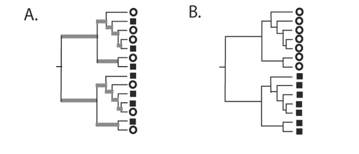
Unifrac index
- Tree representing phylogenetically similar communities, where a significant fraction of the branch length in the tree is shared (gray).
- Tree representing two communities that are maximally different so that 100% of the branch length is unique to either the circle or square environment.
Lozupone C, Knight R2005.UniFrac: a New Phylogenetic Method for Comparing Microbial Communities. Appl Environ Microbiol71:.https://doi.org/10.1128/AEM.71.12.8228-8235.2005
Unifrac index
measures the proportion of the length of the phylogenetic tree specific to either a sample or the other.
\(d_{\text{UF}} = \frac{\sum_{e} l_e \left[ 1_{\{p_e > 0, q_e = 0 \}} + 1_{\{q_e > 0, p_e = 0 \}} \right] }{\sum_{e} l_e \times 1_{\{p_e + q_e > 0 \}}}\)
For each branch \(e\), note \(l_e\) its length and \(p_e\) (resp. \(q_e\)) the fraction of community \(A\) (resp. community \(B\)) below branch \(e\).
Focus on shared taxa
- Unifrac = 0 when all tree branches are shared (abundances can vary)
- Unifrac = 1 when all tree branches are specific
Weighted-Unifrac index
measures the proportion of the length of the phylogenetic tree specific to a sample, weighted by the abundance differences.
\({\text{wUF}} = \frac{\sum_{e} l_e | p_e - q_e| }{\sum_{e} l_e (p_e + q_e)}\)
For each branch \(e\), note \(l_e\) its length and \(p_e\) (resp. \(q_e\)) the fraction of community \(A\) (resp. community \(B\)) below branch \(e\).
Focus on shared taxa
- Weighted-Unifrac = 0 when all ASV are shared with the same abundances
- Weighted-Unifrac = 1 when all ASV are specific and have no tree branch in common
Caracteristics of \(\beta\) diversity (1/2)
| No phylogeny |
Jaccard |
Bray-Curtis |
| With phylogeny |
Unifrac |
Weigthed-Unifrac |
- Jaccard lower than Bray-Curtis ⇒ abondant taxa are not shared
- Jaccard higher than Unifrac ⇒ communities’ taxa are distinct but phylogenetically related
- Unifrac higher than weighted Unifrac ⇒ abondant taxa in both communities are phylogenetically close.
Caracteristics of \(\beta\) diversity (2/2)
In general, qualitative diversities are most sensitive to factors that affect presence/absence of organisms (such as pH, salinity, depth, etc) and therefore useful to study and define bioregions (regions with little of no flow between them)…
… whereas quantitative distances focus on factors that affect relative changes (seasonal changes, nutrient availability, concentration of oxygen, depth, etc) and therefore useful to monitor communities over time or along an environmental gradient.
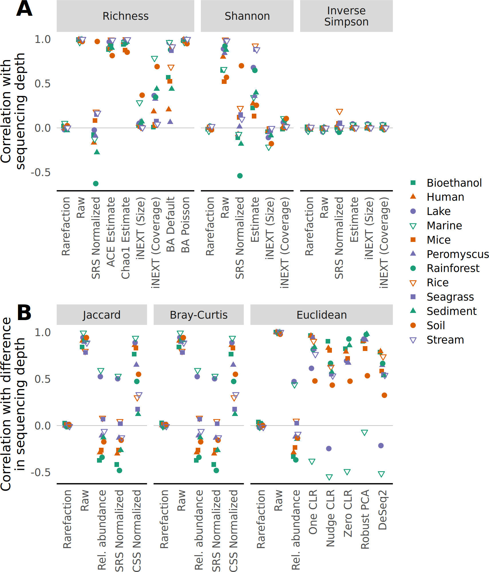
\(\beta\) diversity - rarefaction
best approach to control for uneven sequencing effort
Schloss PD. 2024. Rarefaction is currently the best approach to control for uneven sequencing effort in amplicon sequence analyses. mSphere 9:e00354-23. https://doi.org/10.1128/msphere.00354-23
Practice
Consider working with rarefied data
- Produce \(\beta\) diversity table
- Draw \(\beta\) diversity heatmaps
Visualisation MDS or PCoA plots
Multi-Dimensional Scaling (MDS), also named Principal Coordinate Analysis (PCoA)
Aim: find a lower dimensional representation of the data such that the most information is retained.
- Construct a matrix of pairwise dissimilarities D between each pair of samples (Jaccard, Bray-Curtis dissimilarity, UniFrac distance…).
- Find the first principal coordinates (PCs) that best preserve the original distribution of distances.
MDS or PCoA plots
PCoA focuses on inter-sample dissimilarities
- Each point corresponds to a separate sample
- The coordinates of each point (sample) are determined by the value of the PCs (projection)
- % of variance explained on each axis.
Advantages MDS or PCoA plots
- Based on Non-Euclidean Metrics: Bray-Curtis, Jaccard, UniFrac, Aitchison distance…
- Each PCoA axis is accompanied by the proportion of explained variance, which indicates the extent to which a reduced-dimension projection reflects the original data.
- Compare communities samples/across environmental factors to gain deeper insights into biodiversity patterns.
- The influence of these factors will be assessed using a Permutational Multivariate ANOVA (PERMANOVA).
Practice
- Create PCoA plots by varying the dissimilarity matrix.
- What environmental factors structure the dataset?
- What percentage of the variance is explained?
\(\beta\) diversity partitioning
Test the differences in the community composition of communities (beta diversity) from different groups using a distance matrix,
with the assumption of homogeneous dispersions.
PERMANOVA (1/2)
Permutational Multivariate ANOVA (PERMANOVA) compares the variation between groups to the variation within groups.
Three partitions of the variation
- Total variation (total sum of squares, SST), SST = SSB + SSW
- Variation within groups (sum of squares within groups, SSW)
- Variation between groups (sum of squares between groups, SSB)
PERMANOVA (2/2)
- The significance of the pseudo- F statistic (on the between/within- groups ratio) is evaluated by simulating the null distribution from permutations, with to the design.
- p-values are computed using these permutations.
Limitations
- determining the most suitable distance matrix remains challenging
- it requires permutation to establish its significance, which can be computationally expensive
Practice
- Based on the experimental design (sample_data, metadata), formulate biological questions and write the corresponding statistical model.
- Which dissimilarity matrices are most suitable for community composition of communities?
- Which factors impact \(\beta\) diversity?