RNA-seq transcriptome analysis

Study of chorioallantoic membrane of chicken embryos

RNA-Seq

Author

Affiliation

Christelle Hennequet-Antier

Migale bioinformatics faciliy

Published

June 21, 2024

Modified

June 20, 2025

Introduction

This vignette supports the differential analysis and the functional enrichment test of the dataset described in the data paper entitled “RNA-seq dataset of the chorioallantoic membrane of males and females chicken embryos, after 11 and 15 days of incubation” [1].

Setup

R Packages installed for these analyses.

library(edgeR) # analysis of digital gene expression
library(kableExtra) # construct complex table 
library(magrittr) # provides the pipe operator
library(dplyr) # grammar of data manipulation
library(ggplot2) # data visualisation
library(stringr) # string operators
library(ViSEAGO) # enrichment test

Dataset

This dataset contains the gene expression of chorioallantoic membrane (CAM) of male and female chicken embryos, after 11 and 15 days of incubation. To easy manipulate data, a DGEList objectwas constructed. It contains a matrix counts, a data.frame samples describing the samples and the informations about sequencing, and a data.frame genes containing annotation for the genes obtained using biomaRt R package, with GRCg6a chicken assembly (Ensembl release 106).

# read dge object
dge <- readRDS("./cam-data/cam_dge_tuto.rds")
dge

An object of class "DGEList"
$samples
                       files  group lib.size norm.factors    labels stade
1 Readcount_Ech_C11_F_11.txt EID11F 34020303            1 EID11F_11 EID11
2 Readcount_Ech_C11_F_20.txt EID11F 39748001            1 EID11F_20 EID11
3 Readcount_Ech_C11_F_22.txt EID11F 40176549            1 EID11F_22 EID11
4 Readcount_Ech_C11_F_26.txt EID11F 34417922            1 EID11F_26 EID11
5 Readcount_Ech_C11_F_29.txt EID11F 40019118            1 EID11F_29 EID11
     sex num_sample
1 Female         11
2 Female         20
3 Female         22
4 Female         26
5 Female         29
34 more rows ...

$counts
                    Samples
Tags                 C11_F_11 C11_F_20 C11_F_22 C11_F_26 C11_F_29 C11_F_3
  ENSGALG00000000011     1004     1212      982      967     1166     795
  ENSGALG00000000038        0        0        0        0        0       9
  ENSGALG00000000044        7       32      114       71      165       9
  ENSGALG00000000048     6430     5351     8774     7411    10834    4672
  ENSGALG00000000055     3531     3457     3277     2889     3506    2353
                    Samples
Tags                 C11_F_39 C11_F_41 C11_F_46 C11_F_6 C11_M_14 C11_M_16
  ENSGALG00000000011      795      886      947    1137      914      973
  ENSGALG00000000038        0        5        0       6        5        0
  ENSGALG00000000044       15       53       70      60       33       22
  ENSGALG00000000048     5425    11509     6604    3627     5262     5040
  ENSGALG00000000055     3067     3042     2821    3230     2959     2649
                    Samples
Tags                 C11_M_2 C11_M_24 C11_M_27 C11_M_38 C11_M_44 C11_M_48
  ENSGALG00000000011    1033      947      959     1207     1097      997
  ENSGALG00000000038       0        1        1        0        6        1
  ENSGALG00000000044      23      100      106      177      272       62
  ENSGALG00000000048    4823     7309     4772     8812     9016     9904
  ENSGALG00000000055    2910     2954     2971     3256     3318     2671
                    Samples
Tags                 C11_M_7 C11_M_9 C15_F_102 C15_F_54 C15_F_59 C15_F_64
  ENSGALG00000000011     852    1182       871      881     1135     1336
  ENSGALG00000000038       0       0         1        1        1        1
  ENSGALG00000000044      11      35        85       19        3        3
  ENSGALG00000000048    5887    3631     29829    23884    45168    55303
  ENSGALG00000000055    2525    3296      2796     2941     3664     4334
                    Samples
Tags                 C15_F_70 C15_F_74 C15_F_79 C15_F_88 C15_F_95 C15_M_100
  ENSGALG00000000011      869      825      844      679      960       789
  ENSGALG00000000038        0        0        0        2        1         0
  ENSGALG00000000044       30       15        6        1        9        13
  ENSGALG00000000048    26385    30697    33933    30393    56321     38938
  ENSGALG00000000055     3107     2948     2760     3033     3959      3010
                    Samples
Tags                 C15_M_52 C15_M_57 C15_M_67 C15_M_72 C15_M_76 C15_M_81
  ENSGALG00000000011      939      775     1113      817      786      936
  ENSGALG00000000038        0        7        1        0        0        2
  ENSGALG00000000044        4       15       16        6        6       10
  ENSGALG00000000048    44870    13048    25992    20599    33184    46262
  ENSGALG00000000055     3169     2961     3151     2878     3428     4027
                    Samples
Tags                 C15_M_86 C15_M_93 C15_M_98
  ENSGALG00000000011      860      846      782
  ENSGALG00000000038        1        5        4
  ENSGALG00000000044       12        4        9
  ENSGALG00000000048    32289    38850    44653
  ENSGALG00000000055     2986     2871     3092
26146 more rows ...

$genes
             gene_id external_gene_name
1 ENSGALG00000000011           C10orf88
2 ENSGALG00000000038              CTRB2
3 ENSGALG00000000044            WFIKKN1
4 ENSGALG00000000048                   
5 ENSGALG00000000055            LAMTOR3
                                                                                                        description
1                                           chromosome 10 open reading frame 88 [Source:HGNC Symbol;Acc:HGNC:25822]
2                                                                 chymotrypsinogen B2 [Source:NCBI gene;Acc:431235]
3 WAP, follistatin/kazal, immunoglobulin, kunitz and netrin domain containing 1 [Source:HGNC Symbol;Acc:HGNC:30912]
4                                       V-type proton ATPase catalytic subunit A-like [Source:NCBI gene;Acc:776719]
5                         late endosomal/lysosomal adaptor, MAPK and MTOR activator 3 [Source:NCBI gene;Acc:425210]
  hgnc_symbol chromosome_name
1    C10orf88               6
2                          11
3     WFIKKN1              14
4                          25
5                           4
26146 more rows ...

# convert variables into factors
dge$samples <- dge$samples %>%
  mutate(group = as.factor(group),
         sex = as.factor(sex),
         stade = as.factor(stade))

In this study, the effect of stade with (EID11, EID15) levels and sex with (Female, Male) levels will be explore. The number of biological repetitions is 10, 10, 9, 10 for EID11F, EID11M, EID15F, EID15M, respectively. As mentioned in the paper, the sample numbered 83 (EID15 female) was removed.

The data.frame samples contains a column lib.size for the library size or sequencing depth for each sample, equal to the sum of the aligned reads.

Differential analysis

Statistical analyses were performed using edgeR [2] package to identify differentially expressed genes between CAM from males and CAM from females at incubation day 11 and incubation day 15.

Genes with very low counts across all libraries may be filtered.

# Filter gene with low count, at least number of biological replicates with cpm > valfilt 
valfilt <- 1
nbrepbio <- min(table(dge$samples$group))
keep <- rowSums(edgeR::cpm(dge) > valfilt) >= nbrepbio
dge <- dge[keep, , keep.lib.sizes = FALSE]
dim(dge)

[1] 15124    39

The filtering on genes is based on count per million (cpm) greater than 1 in at least 9 samples corresponding to the minimum number of biological replicates. We kept 15124 expressed genes for further analyses from 39 samples.

Normalisation

A normalization factor is calculated to take into account the different sizes of the sequencing banks (i.e. the total read count) and the distribution of reads per sample on sequencing run, as discussed [3]. Normalization by trimmed mean of M values (TMM) [2] is performed by using the calcNormFactors function from edgeR R package. It calculates a set of normalization factors, one for each sample, to eliminate composition biases between libraries.

Here, the table contains library size and normalisation factors using TMM method ordered by library size. There are also some useful graphs to support the quality control performed during the sequencing steps and bioinformatics analyses.

dge <- calcNormFactors(dge)
dge$samples[order(dge$samples$lib.size), ] %>% 
  kbl() %>% 
  kable_styling() %>% 
  scroll_box(width = "100%", height = "200px")

	files	group	lib.size	norm.factors	labels	stade	sex	num_sample
6	Readcount_Ech_C11_F_3.txt	EID11F	28239877	0.9707889	EID11F_3	EID11	Female	3
12	Readcount_Ech_C11_M_16.txt	EID11M	30753266	0.9678185	EID11M_16	EID11	Male	16
27	Readcount_Ech_C15_F_79.txt	EID15F	30829131	1.0158022	EID15F_79	EID15	Female	79
7	Readcount_Ech_C11_F_39.txt	EID11F	30988543	1.0123821	EID11F_39	EID11	Female	39
19	Readcount_Ech_C11_M_7.txt	EID11M	31208638	0.9970126	EID11M_7	EID11	Male	7
21	Readcount_Ech_C15_F_102.txt	EID15F	32221501	0.9802677	EID15F_102	EID15	Female	102
34	Readcount_Ech_C15_M_72.txt	EID15M	32432332	1.0073170	EID15M_72	EID15	Male	72
11	Readcount_Ech_C11_M_14.txt	EID11M	32899106	0.9673810	EID11M_14	EID11	Male	14
9	Readcount_Ech_C11_F_46.txt	EID11F	33353072	1.0178110	EID11F_46	EID11	Female	46
8	Readcount_Ech_C11_F_41.txt	EID11F	33622506	1.0429180	EID11F_41	EID11	Female	41
1	Readcount_Ech_C11_F_11.txt	EID11F	33981408	0.9898948	EID11F_11	EID11	Female	11
37	Readcount_Ech_C15_M_86.txt	EID15M	34166458	1.0071100	EID15M_86	EID15	Male	86
39	Readcount_Ech_C15_M_98.txt	EID15M	34220625	0.9887918	EID15M_98	EID15	Male	98
30	Readcount_Ech_C15_M_100.txt	EID15M	34249920	1.0060331	EID15M_100	EID15	Male	100
38	Readcount_Ech_C15_M_93.txt	EID15M	34270870	0.9919875	EID15M_93	EID15	Male	93
4	Readcount_Ech_C11_F_26.txt	EID11F	34369303	1.0599808	EID11F_26	EID11	Female	26
22	Readcount_Ech_C15_F_54.txt	EID15F	34403366	1.0024428	EID15F_54	EID15	Female	54
28	Readcount_Ech_C15_F_88.txt	EID15F	34515320	1.0000987	EID15F_88	EID15	Female	88
15	Readcount_Ech_C11_M_27.txt	EID11M	34704465	1.0311382	EID11M_27	EID11	Male	27
18	Readcount_Ech_C11_M_48.txt	EID11M	35116336	1.0623694	EID11M_48	EID11	Male	48
26	Readcount_Ech_C15_F_74.txt	EID15F	35566461	0.9961322	EID15F_74	EID15	Female	74
31	Readcount_Ech_C15_M_52.txt	EID15M	35666960	0.9866407	EID15M_52	EID15	Male	52
25	Readcount_Ech_C15_F_70.txt	EID15F	35711970	1.0172644	EID15F_70	EID15	Female	70
13	Readcount_Ech_C11_M_2.txt	EID11M	35760262	0.9711445	EID11M_2	EID11	Male	2
20	Readcount_Ech_C11_M_9.txt	EID11M	36244024	0.9700712	EID11M_9	EID11	Male	9
35	Readcount_Ech_C15_M_76.txt	EID15M	36423127	1.0053627	EID15M_76	EID15	Male	76
10	Readcount_Ech_C11_F_6.txt	EID11F	36634581	0.9163450	EID11F_6	EID11	Female	6
32	Readcount_Ech_C15_M_57.txt	EID15M	36729326	1.0033506	EID15M_57	EID15	Male	57
14	Readcount_Ech_C11_M_24.txt	EID11M	38256961	1.0244010	EID11M_24	EID11	Male	24
33	Readcount_Ech_C15_M_67.txt	EID15M	38400121	0.9927465	EID15M_67	EID15	Male	67
36	Readcount_Ech_C15_M_81.txt	EID15M	38612243	0.9411493	EID15M_81	EID15	Male	81
16	Readcount_Ech_C11_M_38.txt	EID11M	39030485	1.0348989	EID11M_38	EID11	Male	38
17	Readcount_Ech_C11_M_44.txt	EID11M	39274952	1.0553474	EID11M_44	EID11	Male	44
2	Readcount_Ech_C11_F_20.txt	EID11F	39700690	0.9793198	EID11F_20	EID11	Female	20
5	Readcount_Ech_C11_F_29.txt	EID11F	39971511	1.0200657	EID11F_29	EID11	Female	29
3	Readcount_Ech_C11_F_22.txt	EID11F	40117899	1.0346771	EID11F_22	EID11	Female	22
23	Readcount_Ech_C15_F_59.txt	EID15F	40729955	0.9517567	EID15F_59	EID15	Female	59
29	Readcount_Ech_C15_F_95.txt	EID15F	43711444	0.9940782	EID15F_95	EID15	Female	95
24	Readcount_Ech_C15_F_64.txt	EID15F	49181211	1.0044379	EID15F_64	EID15	Female	64

# barplot of scaling factors
p<-ggplot(dge$samples, aes(x=dge$samples$labels, y=dge$samples$norm.factors, fill=dge$samples$group)) +
    geom_col() + xlab("Samples") + ylab("TMM factors") + labs(fill = "group") + theme_bw() +
    theme(axis.text.x = element_text(angle=90)) + ggtitle("TMM size factors \n")
p

# barplot of library size with group information
p<-ggplot(dge$samples, aes(x=dge$samples$labels, y=dge$samples$lib.size, fill=dge$samples$group)) +
    geom_col() + xlab("Samples") + ylab("Library size") + labs(fill = "group") + theme_bw() +
    theme(axis.text.x = element_text(angle=90)) + ggtitle("Library size \n")
p

Multidimensional scaling plot

Multidimensional scaling (MDS) plot shows the relationships between the samples. The top (500 genes) are used to calculate the distance between expression profiles of samples. The distance approximate the log2 fold change between the samples.

As expected, samples are grouped by stade and sex.

limma::plotMDS(dge, col = as.numeric(dge$samples$group), labels = dge$samples$num_sample, cex=0.9, gene.selection = "pairwise", top = 500, main = "MDS plot with top 500 genes")
legend("topleft", legend = levels(dge$samples$group), col = unique(as.numeric(dge$samples$group)),
        cex = 0.8, lwd = 1)

Differential analysis

The aim is to identify the genes differentially expressed between sex at each day of incubation (stade variable). At this step, read counts were normalized using trimmed mean of M-values (TMM) method [2] from edgeR R package. The differential analysis is based on a Generalized Linear Model (GLM) to take into account the distribution of count-type data (non-normality of the data) and over-dispersion. The GLM model [4] was fitted with one factor of four levels: EID11F, EID11M, EID15F, EID15M.

First, the matrix design was computed.

#matrix design: one factor group
design <- model.matrix(~ 0 + group, data = dge$samples)
colnames(design) <- colnames(design) %>% str_remove(., "group")
design

   EID11F EID11M EID15F EID15M
1       1      0      0      0
2       1      0      0      0
3       1      0      0      0
4       1      0      0      0
5       1      0      0      0
6       1      0      0      0
7       1      0      0      0
8       1      0      0      0
9       1      0      0      0
10      1      0      0      0
11      0      1      0      0
12      0      1      0      0
13      0      1      0      0
14      0      1      0      0
15      0      1      0      0
16      0      1      0      0
17      0      1      0      0
18      0      1      0      0
19      0      1      0      0
20      0      1      0      0
21      0      0      1      0
22      0      0      1      0
23      0      0      1      0
24      0      0      1      0
25      0      0      1      0
26      0      0      1      0
27      0      0      1      0
28      0      0      1      0
29      0      0      1      0
30      0      0      0      1
31      0      0      0      1
32      0      0      0      1
33      0      0      0      1
34      0      0      0      1
35      0      0      0      1
36      0      0      0      1
37      0      0      0      1
38      0      0      0      1
39      0      0      0      1
attr(,"assign")
[1] 1 1 1 1
attr(,"contrasts")
attr(,"contrasts")$group
[1] "contr.treatment"

Genes differentially expressed between CAM males and females were obtained for each incubation day using the likelihood ratio test on the two defined contrasts EID11_MvsF = EID11M - EID11F and EID15_MvsF = EID15M - EID15F.

# differences between sex (M versus F) within EID11
EID11_MvsF <- makeContrasts(EID11M - EID11F, levels=colnames(design))
# differences between sex (M versus F) within EID15
EID15_MvsF <- makeContrasts(EID15M - EID15F, levels=colnames(design))

my.contrasts <- list(EID11_MvsF = EID11_MvsF, 
                     EID15_MvsF = EID15_MvsF)

We set robust=TRUE when estimating the dispersion. This has no effect on the downstream analysis, but is nevertheless very useful for identifying outliers from the trend of the mean dispersion of the negative binomial distribution.

# robust at gene level
# with specific design
dge<-estimateDisp(dge, design = design, robust=TRUE)
#summary(dge$tagwise.dispersion)
plotBCV(dge)

We used GLM model [4] to perform likelihood ratio tests for each contrast defined as EID11_MvsF, EID15_MvsF. List of differentially expressed genes were obtained after controlling the false positive rate with a Benjamini-Hochberg correction [5] at 0.05 threshold.

# model GLM with the design
fit <- glmFit(dge, design = design)

EID11_MvsF
EID15_MvsF

lrt <- glmLRT(fit, contrast = EID11_MvsF)
# Number of DE genes
summary(decideTests(lrt))

       -1*EID11F 1*EID11M
Down                  157
NotSig              14525
Up                    442

# Table of DE genes results
res <- topTags(lrt, n=nrow(dge$counts), adjust.method="BH", sort.by="none")$table
# see the first rows
head(res)

                              gene_id external_gene_name
ENSGALG00000000011 ENSGALG00000000011           C10orf88
ENSGALG00000000044 ENSGALG00000000044            WFIKKN1
ENSGALG00000000048 ENSGALG00000000048                   
ENSGALG00000000055 ENSGALG00000000055            LAMTOR3
ENSGALG00000000059 ENSGALG00000000059              TUBB3
ENSGALG00000000067 ENSGALG00000000067                SPR
                                                                                                                         description
ENSGALG00000000011                                           chromosome 10 open reading frame 88 [Source:HGNC Symbol;Acc:HGNC:25822]
ENSGALG00000000044 WAP, follistatin/kazal, immunoglobulin, kunitz and netrin domain containing 1 [Source:HGNC Symbol;Acc:HGNC:30912]
ENSGALG00000000048                                       V-type proton ATPase catalytic subunit A-like [Source:NCBI gene;Acc:776719]
ENSGALG00000000055                         late endosomal/lysosomal adaptor, MAPK and MTOR activator 3 [Source:NCBI gene;Acc:425210]
ENSGALG00000000059                                                           tubulin, beta 3 class III [Source:NCBI gene;Acc:431043]
ENSGALG00000000067                   sepiapterin reductase (7,8-dihydrobiopterin:NADP+ oxidoreductase) [Source:NCBI gene;Acc:425255]
                   hgnc_symbol chromosome_name       logFC    logCPM        LR
ENSGALG00000000011    C10orf88               6  0.02516631 4.7368237 0.1103700
ENSGALG00000000044     WFIKKN1              14  0.45759194 0.3106141 0.7125593
ENSGALG00000000048                          25 -0.15043214 9.1528049 0.6450647
ENSGALG00000000055                           4 -0.09488628 6.4495919 2.7667930
ENSGALG00000000059                          11  0.41117847 7.8279704 2.8421317
ENSGALG00000000067         SPR               4  0.09039913 4.5458272 1.0399541
                       PValue       FDR
ENSGALG00000000011 0.73972326 0.9886434
ENSGALG00000000044 0.39859549 0.9436440
ENSGALG00000000048 0.42188272 0.9544246
ENSGALG00000000055 0.09623880 0.6636528
ENSGALG00000000059 0.09182232 0.6591022
ENSGALG00000000067 0.30783215 0.9078363

Histogram of raw p-values and mean-difference plot (also called MA-plot) are useful graphs to validate the model.

 # histogram of raw pvalues
 p <- ggplot(data = lrt$table, aes(x = PValue))
 p <- p + geom_histogram(color="darkblue", fill="lightblue")
 p <- p + theme_bw() + xlab("Raw pvalue")
 p <- p + ggtitle("Histogram of raw pvalues for EID11_MvsF")
 print(p)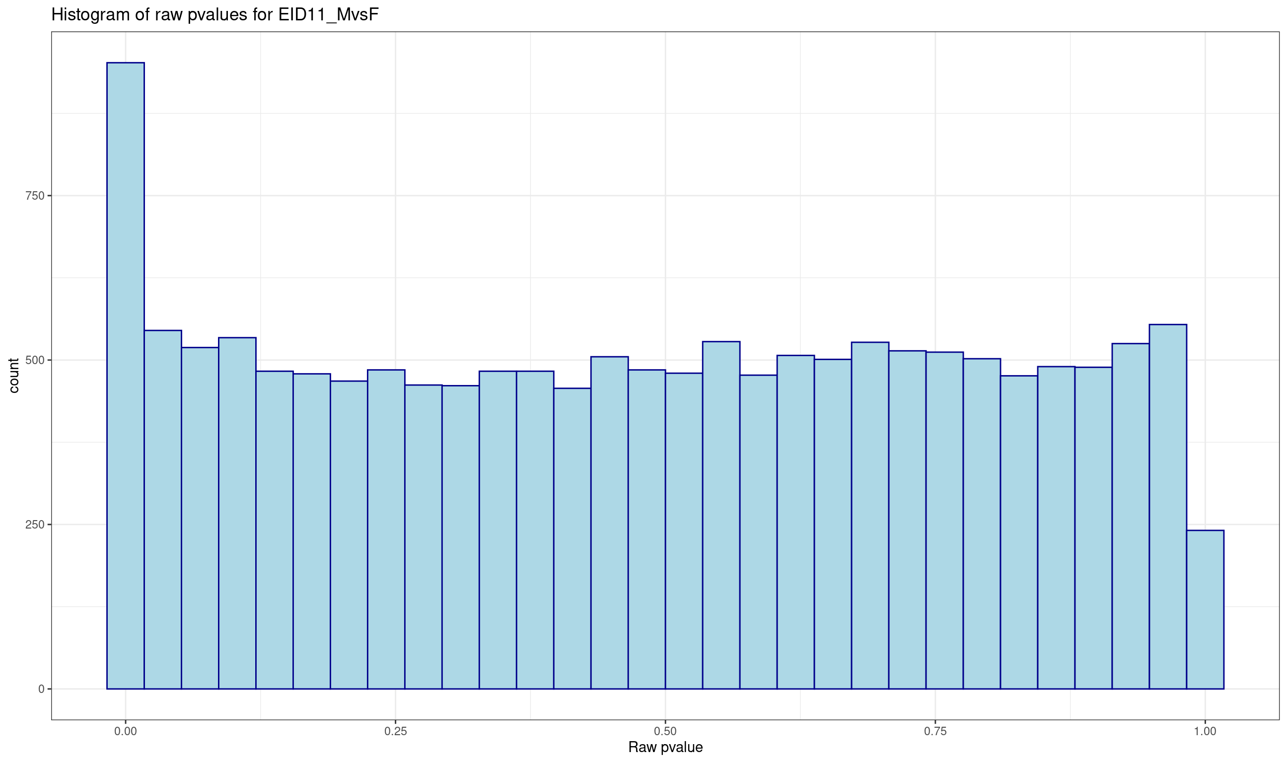

# MA plot
 plotMD(lrt, main = "MA plot for EID11_MvsF")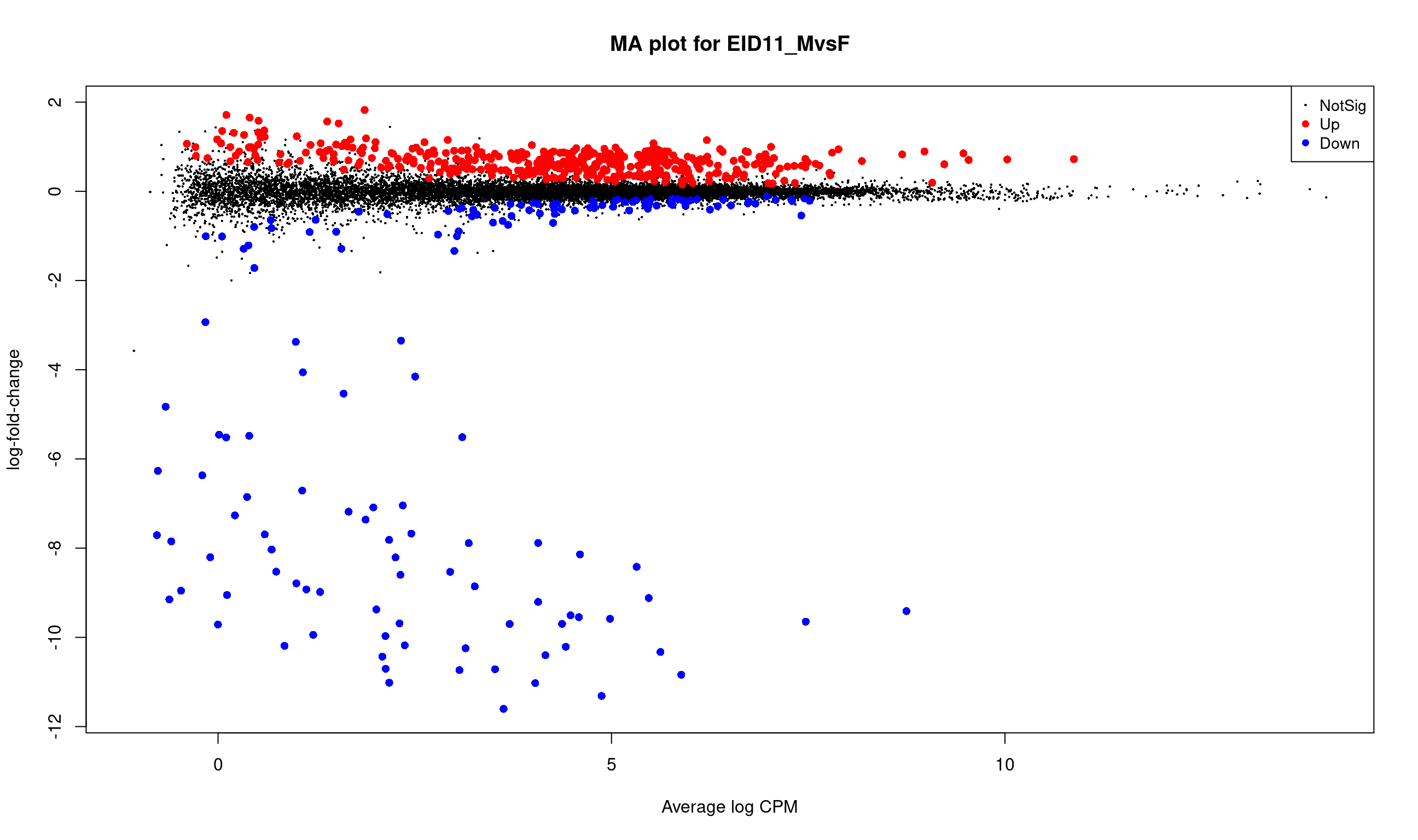

Volcano plots represent a useful way to visualise the results of differential expression analyses. The x-axis is log2 fold change and represents biological significance. The y-axis is -Log10 Pvalue of the contrast tested and represents statistical significance. The highest genes on the graph are the most significantly differentially expressed (DE) genes.

The EnhancedVolcano R package offers new functionalities to produce publication-ready volcano plots.

# volcano plot
 p <- ggplot(data = res, aes(x = logFC, y = -log10(FDR)))
 p <- p +  geom_point(size=2, shape=19)
 p <- p + ggtitle("Volcanoplot: Difference between males and females at EID11")
 p

Save the results in separated files using a comma for the decimal point and a semicolon for the separator between columns.

# complete - all genes after filtering step
EID11_MvsF_bg  <- res
write.csv2(EID11_MvsF_bg, file="output/complete_EID11_males_vs_females.csv")
# up regulated DE genes at FDR threshold 0.05
EID11_MvsF_up <- dplyr::filter(res, FDR <= 0.05 & logFC > 0)
write.csv2(EID11_MvsF_up, file="output/up_EID11_males_vs_females.csv")
# down regulated DE genes at FDR threshold 0.05
EID11_MvsF_down <- dplyr::filter(res, FDR <= 0.05 & logFC < 0)
write.csv2(EID11_MvsF_down, file="output/down_EID11_males_vs_females.csv")

lrt <- glmLRT(fit, contrast = EID15_MvsF)
# Number of DE genes
summary(decideTests(lrt))

       -1*EID15F 1*EID15M
Down                  134
NotSig              14551
Up                    439

# Table of DE genes results
res <- topTags(lrt, n=nrow(dge$counts), adjust.method="BH", sort.by="none")$table
# see the first rows
head(res)

                              gene_id external_gene_name
ENSGALG00000000011 ENSGALG00000000011           C10orf88
ENSGALG00000000044 ENSGALG00000000044            WFIKKN1
ENSGALG00000000048 ENSGALG00000000048                   
ENSGALG00000000055 ENSGALG00000000055            LAMTOR3
ENSGALG00000000059 ENSGALG00000000059              TUBB3
ENSGALG00000000067 ENSGALG00000000067                SPR
                                                                                                                         description
ENSGALG00000000011                                           chromosome 10 open reading frame 88 [Source:HGNC Symbol;Acc:HGNC:25822]
ENSGALG00000000044 WAP, follistatin/kazal, immunoglobulin, kunitz and netrin domain containing 1 [Source:HGNC Symbol;Acc:HGNC:30912]
ENSGALG00000000048                                       V-type proton ATPase catalytic subunit A-like [Source:NCBI gene;Acc:776719]
ENSGALG00000000055                         late endosomal/lysosomal adaptor, MAPK and MTOR activator 3 [Source:NCBI gene;Acc:425210]
ENSGALG00000000059                                                           tubulin, beta 3 class III [Source:NCBI gene;Acc:431043]
ENSGALG00000000067                   sepiapterin reductase (7,8-dihydrobiopterin:NADP+ oxidoreductase) [Source:NCBI gene;Acc:425255]
                   hgnc_symbol chromosome_name       logFC    logCPM
ENSGALG00000000011    C10orf88               6 -0.03122908 4.7368237
ENSGALG00000000044     WFIKKN1              14 -1.05217055 0.3106141
ENSGALG00000000048                          25 -0.01456782 9.1528049
ENSGALG00000000055                           4  0.02539276 6.4495919
ENSGALG00000000059                          11 -0.23793501 7.8279704
ENSGALG00000000067         SPR               4  0.09422590 4.5458272
                            LR     PValue       FDR
ENSGALG00000000011 0.159739642 0.68939634 0.9996332
ENSGALG00000000044 3.318413100 0.06850793 0.6500799
ENSGALG00000000048 0.005742689 0.93959370 0.9996332
ENSGALG00000000055 0.188175870 0.66443918 0.9996332
ENSGALG00000000059 0.906407523 0.34106941 0.9996332
ENSGALG00000000067 1.058917896 0.30346212 0.9955664

Histogram of raw p-values and mean-difference plot (also called MA-plot) are useful graphs to validate the model.

 # histogram of raw pvalues
 p <- ggplot(data = lrt$table, aes(x = PValue))
 p <- p + geom_histogram(color="darkblue", fill="lightblue")
 p <- p + theme_bw() + xlab("Raw pvalue")
 p <- p + ggtitle("Histogram of raw pvalues for EID15_MvsF")
 print(p)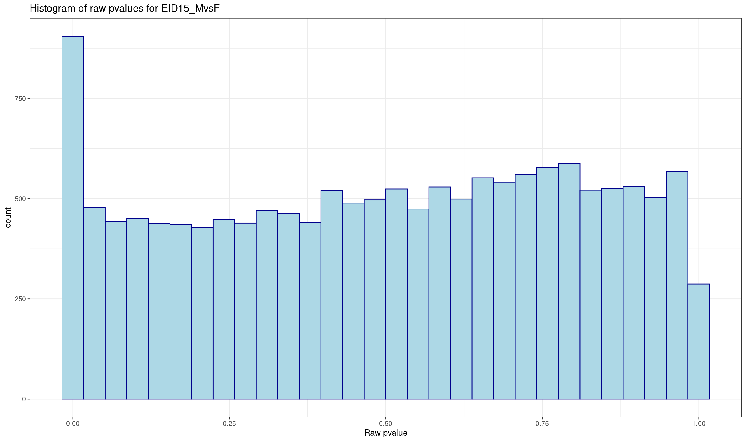

# MA plot
plotMD(lrt, main = "MA plot for EID15_MvsF")

See also the EnhancedVolcano R package, it offers new functionalities to produce publication-ready volcano plots.

# volcano plot
 p <- ggplot(data = res, aes(x = logFC, y = -log10(FDR)))
 p <- p +  geom_point(size=2, shape=19)
 p <- p + ggtitle("Volcanoplot: Difference between males and females at EID15")
 p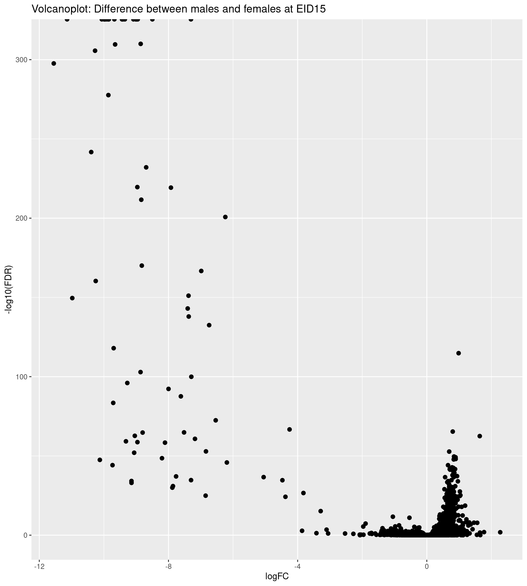

Save the results in separated files using a comma for the decimal point and a semicolon for the separator between columns.

# complete - all genes after filtering step
EID15_MvsF_bg <- res
write.csv2(EID15_MvsF_bg, file="output/complete_EID15_males_vs_females.csv")
# up regulated DE genes at FDR threshold 0.05
EID15_MvsF_up <- dplyr::filter(res, FDR <= 0.05 & logFC > 0)
write.csv2(EID15_MvsF_up, file="output/up_EID15_males_vs_females.csv")
# down regulated DE genes at FDR threshold 0.05
EID15_MvsF_down <- dplyr::filter(res, FDR <= 0.05 & logFC < 0)
write.csv2(EID15_MvsF_down, file="output/down_EID15_males_vs_females.csv")

Functional enrichment test

The comparison of biological processes (BP) between the lists of DE genes were performed using ViSEAGO R package [6].

Genes of interest

The results from differential analysis were used.

# Use a common background for EID11 et EID15 analyses
background <- unique(EID11_MvsF_bg$gene_id, EID15_MvsF_bg$gene_id) 
DE_EID11_MvsF_up <- EID11_MvsF_up$gene_id[stringr::str_starts(EID11_MvsF_up$gene_id, "ENSGALG")] 
DE_EID11_MvsF_down <- EID11_MvsF_down$gene_id[stringr::str_starts(EID11_MvsF_down$gene_id, "ENSGALG")]
DE_EID15_MvsF_up <- EID15_MvsF_up$gene_id[stringr::str_starts(EID15_MvsF_up$gene_id, "ENSGALG")]
DE_EID15_MvsF_down <- EID15_MvsF_down$gene_id[stringr::str_starts(EID15_MvsF_down$gene_id, "ENSGALG")]

GO annotation of genes

The genes were previously annotated using biomaRt R package, with GRCg6a chicken assembly (Ensembl release 106).

# load GO annotations from Ensembl
load("./cam-data/CAM_myGENE2GO_Ensembl.RData")
myGENE2GO_Ensembl

- object class: gene2GO
- database: Ensembl
- stamp/version: genes  Ensembl Genes 106
- organism id: ggallus_gene_ensembl

GO annotations:
- Molecular Function (MF): 12702 annotated genes with 41502 terms (3406 unique terms)
- Biological Process (BP): 12653 annotated genes with 75167 terms (9994 unique terms)
- Cellular Component (CC): 12096 annotated genes with 43282 terms (1501 unique terms)

Functionnal GO enrichment tests

At this step, we used myGENE2GO directly from Ensembl query. For each list of genes of interest, the GO enrichment tests were performed for BP category with Fisher’s exact test based on a common background of genes (all genes expressed in the study). The number minimal of genes is set to the value of nodeSize to consider valuable GO term.

# create topGOdata for BP
BP_EID11_MvsF_up <-ViSEAGO::create_topGOdata(
  geneSel = DE_EID11_MvsF_up,
  allGenes = background,
  gene2GO = myGENE2GO_Ensembl, 
  ont = "BP",
  nodeSize = 5
)

BP_EID11_MvsF_down <-ViSEAGO::create_topGOdata(
  geneSel = DE_EID11_MvsF_down,
  allGenes = background,
  gene2GO = myGENE2GO_Ensembl, 
  ont = "BP",
  nodeSize = 5
)

BP_EID15_MvsF_up <-ViSEAGO::create_topGOdata(
  geneSel = DE_EID15_MvsF_up,
  allGenes = background,
  gene2GO = myGENE2GO_Ensembl, 
  ont = "BP",
  nodeSize = 5
)

BP_EID15_MvsF_down <-ViSEAGO::create_topGOdata(
  geneSel = DE_EID15_MvsF_down,
  allGenes = background,
  gene2GO = myGENE2GO_Ensembl, 
  ont = "BP",
  nodeSize = 5
)

# perform TopGO test using clasic algorithm
classic_EID11_MvsF_up <-topGO::runTest(
  BP_EID11_MvsF_up,
  algorithm ="classic",
  statistic = "fisher"
)

classic_EID11_MvsF_down <-topGO::runTest(
  BP_EID11_MvsF_down,
  algorithm ="classic",
  statistic = "fisher"
)

classic_EID15_MvsF_up <-topGO::runTest(
  BP_EID15_MvsF_up,
  algorithm ="classic",
  statistic = "fisher"
)

classic_EID15_MvsF_down <-topGO::runTest(
  BP_EID15_MvsF_down,
  algorithm ="classic",
  statistic = "fisher"
)

classic_EID11_MvsF_up


Description: Ensembl ggallus_gene_ensembl genes  Ensembl Genes 106 
Ontology: BP 
'classic' algorithm with the 'fisher' test
6416 GO terms scored: 17 terms with p < 0.01
Annotation data:
    Annotated genes: 9851 
    Significant genes: 293 
    Min. no. of genes annotated to a GO: 5 
    Nontrivial nodes: 3115

classic_EID11_MvsF_down


Description: Ensembl ggallus_gene_ensembl genes  Ensembl Genes 106 
Ontology: BP 
'classic' algorithm with the 'fisher' test
6416 GO terms scored: 23 terms with p < 0.01
Annotation data:
    Annotated genes: 9851 
    Significant genes: 84 
    Min. no. of genes annotated to a GO: 5 
    Nontrivial nodes: 1553

classic_EID15_MvsF_up


Description: Ensembl ggallus_gene_ensembl genes  Ensembl Genes 106 
Ontology: BP 
'classic' algorithm with the 'fisher' test
6416 GO terms scored: 27 terms with p < 0.01
Annotation data:
    Annotated genes: 9851 
    Significant genes: 292 
    Min. no. of genes annotated to a GO: 5 
    Nontrivial nodes: 3205

classic_EID15_MvsF_down


Description: Ensembl ggallus_gene_ensembl genes  Ensembl Genes 106 
Ontology: BP 
'classic' algorithm with the 'fisher' test
6416 GO terms scored: 15 terms with p < 0.01
Annotation data:
    Annotated genes: 9851 
    Significant genes: 65 
    Min. no. of genes annotated to a GO: 5 
    Nontrivial nodes: 1031

Combine enriched GO terms

The results of enrichment tests were combined in an interactive table. This table contains for each enriched GO terms, additional columns including the list of significant genes and frequency (ratio between the number of significant genes and number of background genes in a specific GO tag) evaluated by comparison.

BP_sResults<-ViSEAGO::merge_enrich_terms(
  Input=base::list(EID11_MvsF_down=base::c("BP_EID11_MvsF_down","classic_EID11_MvsF_down"),
                   EID15_MvsF_down=base::c("BP_EID15_MvsF_down","classic_EID15_MvsF_down"),
                   EID11_MvsF_up=base::c("BP_EID11_MvsF_up","classic_EID11_MvsF_up"),
                   EID15_MvsF_up=base::c("BP_EID15_MvsF_up","classic_EID15_MvsF_up")
                   )
  )

# display the merged table
ViSEAGO::show_table(BP_sResults)

# print the merged table in a file
ViSEAGO::show_table(BP_sResults,"./output/BP_sResults.xls")

Graphs of GO enrichment tests

# count significant (or not) pvalues by condition
ViSEAGO::GOcount(BP_sResults)

GO terms Semantic Similarity

The Semantic Similarity (SS) between enriched GO terms were computed using Wang’s method based on the topology of GO graph structure.

# initialyse 
myGOs<-ViSEAGO::build_GO_SS(gene2GO=myGENE2GO_Ensembl,enrich_GO_terms=BP_sResults)
# compute all available Semantic Similarity (SS) measures
myGOs<-ViSEAGO::compute_SS_distances(myGOs,distance="Wang")

Clustering heatmap of GO terms

A hierarchical clustering was performed using Wang SS distance between enriched GO terms and ward.D2 aggregation criteria. Enriched GO terms are ranked in a dendrogram and colored depending on their cluster assignation. A heatmap of -log10(pvalue) of enrichment test for each comparison and optionally the Information Content (IC) were displayed.

# GOterms heatmap with the default parameters
Wang_clusters_wardD2 <- ViSEAGO::GOterms_heatmap(
  myGOs,
  showIC=T,
  GO.tree=base::list(
    tree=base::list(
      distance="Wang",
      aggreg.method="ward.D2"
    ),
    cut=base::list(
      dynamic=base::list(
        pamStage=T,
        pamRespectsDendro=T,
        deepSplit=2,
        minClusterSize =4)
      )
    ),
  samples.tree=NULL
)

# Display the clusters-heatmap
ViSEAGO::show_heatmap(Wang_clusters_wardD2, "GOterms", plotly_update = TRUE)

# Display the clusters-heatmap table
ViSEAGO::show_table(Wang_clusters_wardD2)

# Print the clusters-heatmap table
ViSEAGO::show_table(
  Wang_clusters_wardD2,
  "./output/cluster_heatmap_Wang_wardD2.xls"
)

Multi Dimensional Scaling of GO terms

The MDS plot allows the user to visualise functional coherence as a whole and interactively explore functional subsets in greater detail.

# display colored MDSplot
ViSEAGO::MDSplot(Wang_clusters_wardD2)

Results

This a summarise of the functional enrichment tests. Due to package updates since the publication, new enriched GO terms have appeared, resulting in slight differences in the heatmap and MDS plots.

print(BP_sResults)

- object class: enrich_GO_terms
- ontology: BP
- method: topGO
- summary:
 EID11_MvsF_down
      BP_EID11_MvsF_down 
        description: Ensembl ggallus_gene_ensembl genes  Ensembl Genes 106
        available_genes: 15124
        available_genes_significant: 124
        feasible_genes: 9851
        feasible_genes_significant: 84
        genes_nodeSize: 5
        nodes_number: 6416
        edges_number: 13970
      classic_EID11_MvsF_down 
        description: Ensembl ggallus_gene_ensembl genes  Ensembl Genes 106 
        test_name: fisher
        algorithm_name: classic
        GO_scored: 6416
        GO_significant: 23
        feasible_genes: 9851
        feasible_genes_significant: 84
        genes_nodeSize: 5
        Nontrivial_nodes: 1553 
 EID15_MvsF_down
      BP_EID15_MvsF_down 
        description: Ensembl ggallus_gene_ensembl genes  Ensembl Genes 106
        available_genes: 15124
        available_genes_significant: 100
        feasible_genes: 9851
        feasible_genes_significant: 65
        genes_nodeSize: 5
        nodes_number: 6416
        edges_number: 13970
      classic_EID15_MvsF_down 
        description: Ensembl ggallus_gene_ensembl genes  Ensembl Genes 106 
        test_name: fisher
        algorithm_name: classic
        GO_scored: 6416
        GO_significant: 15
        feasible_genes: 9851
        feasible_genes_significant: 65
        genes_nodeSize: 5
        Nontrivial_nodes: 1031 
 EID11_MvsF_up
      BP_EID11_MvsF_up 
        description: Ensembl ggallus_gene_ensembl genes  Ensembl Genes 106
        available_genes: 15124
        available_genes_significant: 415
        feasible_genes: 9851
        feasible_genes_significant: 293
        genes_nodeSize: 5
        nodes_number: 6416
        edges_number: 13970
      classic_EID11_MvsF_up 
        description: Ensembl ggallus_gene_ensembl genes  Ensembl Genes 106 
        test_name: fisher
        algorithm_name: classic
        GO_scored: 6416
        GO_significant: 17
        feasible_genes: 9851
        feasible_genes_significant: 293
        genes_nodeSize: 5
        Nontrivial_nodes: 3115 
 EID15_MvsF_up
      BP_EID15_MvsF_up 
        description: Ensembl ggallus_gene_ensembl genes  Ensembl Genes 106
        available_genes: 15124
        available_genes_significant: 410
        feasible_genes: 9851
        feasible_genes_significant: 292
        genes_nodeSize: 5
        nodes_number: 6416
        edges_number: 13970
      classic_EID15_MvsF_up 
        description: Ensembl ggallus_gene_ensembl genes  Ensembl Genes 106 
        test_name: fisher
        algorithm_name: classic
        GO_scored: 6416
        GO_significant: 27
        feasible_genes: 9851
        feasible_genes_significant: 292
        genes_nodeSize: 5
        Nontrivial_nodes: 3205 
 - enrichment pvalue cutoff:
        EID11_MvsF_down : 0.01
        EID15_MvsF_down : 0.01
        EID11_MvsF_up : 0.01
        EID15_MvsF_up : 0.01
- enrich GOs (in at least one list): 51 GO terms of 4 conditions.
        EID11_MvsF_down : 23 terms
        EID15_MvsF_down : 15 terms
        EID11_MvsF_up : 17 terms
        EID15_MvsF_up : 27 terms

Reproducibility token

sessioninfo::session_info(pkgs = "attached")

─ Session info ───────────────────────────────────────────────────────────────
 setting  value
 version  R version 4.4.1 (2024-06-14)
 os       Ubuntu 22.04.4 LTS
 system   x86_64, linux-gnu
 ui       X11
 language (EN)
 collate  fr_FR.UTF-8
 ctype    fr_FR.UTF-8
 tz       Europe/Paris
 date     2024-08-19
 pandoc   3.1.11 @ /usr/lib/rstudio/resources/app/bin/quarto/bin/tools/x86_64/ (via rmarkdown)

─ Packages ───────────────────────────────────────────────────────────────────
 package       * version date (UTC) lib source
 AnnotationDbi * 1.66.0  2024-05-01 [1] Bioconductor 3.19 (R 4.4.0)
 Biobase       * 2.64.0  2024-04-30 [1] Bioconductor 3.19 (R 4.4.0)
 BiocGenerics  * 0.50.0  2024-04-30 [1] Bioconductor 3.19 (R 4.4.0)
 dplyr         * 1.1.4   2023-11-17 [1] CRAN (R 4.4.0)
 edgeR         * 4.2.0   2024-04-30 [1] Bioconductor 3.19 (R 4.4.0)
 ggplot2       * 3.5.1   2024-04-23 [1] CRAN (R 4.4.0)
 GO.db         * 3.19.1  2024-05-21 [1] Bioconductor
 graph         * 1.82.0  2024-04-30 [1] Bioconductor 3.19 (R 4.4.0)
 IRanges       * 2.38.0  2024-04-30 [1] Bioconductor 3.19 (R 4.4.0)
 kableExtra    * 1.4.0   2024-01-24 [1] CRAN (R 4.4.0)
 limma         * 3.60.2  2024-05-19 [1] Bioconductor 3.19 (R 4.4.0)
 magrittr      * 2.0.3   2022-03-30 [1] CRAN (R 4.4.0)
 S4Vectors     * 0.42.0  2024-04-30 [1] Bioconductor 3.19 (R 4.4.0)
 SparseM       * 1.83    2024-05-30 [1] CRAN (R 4.4.0)
 stringr       * 1.5.1   2023-11-14 [1] CRAN (R 4.4.0)
 topGO         * 2.56.0  2024-04-30 [1] Bioconductor 3.19 (R 4.4.0)
 ViSEAGO       * 1.18.0  2024-04-30 [1] Bioconductor 3.19 (R 4.4.0)

 [1] /home/chennequet/R/x86_64-pc-linux-gnu-library/4.4
 [2] /usr/local/lib/R/site-library
 [3] /usr/lib/R/site-library
 [4] /usr/lib/R/library

──────────────────────────────────────────────────────────────────────────────

References

1. Hennequet-Antier C, Halgrain M, Réhault-Godbert S. RNA-seq dataset of the chorioallantoic membrane of male and female chicken embryos, after 11 and 15 days of incubation. Data in Brief. 2024;110830. doi:https://doi.org/10.1016/j.dib.2024.110830.

2. Robinson MD, Oshlack A. A scaling normalization method for differential expression analysis of RNA-seq data. Genome Biology. 2010;11:R25. doi:10.1186/gb-2010-11-3-r25.

3. Dillies M-A, Rau A, Aubert J, Hennequet-Antier C, Jeanmougin M, Servant N, et al. A comprehensive evaluation of normalization methods for illumina high-throughput RNA sequencing data analysis. Brief Bioinform. 2012;14:671–83.

4. Mc DJ, Chen Y, Smyth GK. Differential expression analysis of multifactor RNA-Seq experiments with respect to biological variation. Nucleic Acids Res. 2012;40:4288–97.

5. Benjamini Y, Hochberg Y. Controlling the false discovery rate: A practical and powerful approach to multiple testing. Journal of the Royal Statistical Society Series B (Methodological). 1995;57:289–300. http://www.jstor.org/stable/2346101.

6. Brionne A, Juanchich A, Hennequet-Antier C. ViSEAGO: A bioconductor package for clustering biological functions using gene ontology and semantic similarity. BioData Mining. 2019;12:16. doi:10.1186/s13040-019-0204-1.

A work by Migale Bioinformatics Facility
Université Paris-Saclay, INRAE, MaIAGE, 78350, Jouy-en-Josas, France
Université Paris-Saclay, INRAE, BioinfOmics, MIGALE bioinformatics facility, 78350, Jouy-en-Josas, France