
cd ~/work
mkdir -p FROGS_16S/LOGS
cd FROGS_16S
conda activate sra-tools-2.11.0
awk '{print "fasterq-dump --split-files --progress --force --outdir . --threads 1", $3}' <(grep SRR metadata.tsv) >> download.sh
bash download.sh
conda deactivateMetabarcoding analaysis (16S rRNA marker) with FROGS 4.1.0 in command line
metabarcoding
FROGS
command line
The purpose of this post is to show you how to analyze 16S metabarcoding datasets (Illumina 16S V3-V4 region) from the command line with FROGS front server and how to explore data in a BIOM file with phyloseq
Introduction
FROGS
Note
The analyses performed in this document have been performed on the Migale cluster front.migale.inrae.fr and rstudio.migale.inrae.fr. You can easily reproduce the analyses if you have got an account on our infrastructure. If you are not familiar with the Migale infrastructure, you can read the dedicated post.
Warning
This post is intended neither to provide an in-depth analysis of the dataset nor to answer biological questions (refer to our other tutorial instead). It is rather an illustration of the technical possibilities and various tools offered by the Migale infrastructure for this kind of data. Please be aware that the parameters of the tools used here are tailored to this particular dataset and should be adapted to your own needs
Data
The dataset we will analyze in this post is a part of the samples used in this publication. These are 16S rRNA amplicons of meat and seafood products, as well as synthetic communities, sequenced with the Illumina MiSeq sequencing technology.
The following table gives information on samples, commonly refereed to as metadata and stored in a metadata file:
Bioinformatics analyses
Get and prepare data
The first step is to get the FASTQ files, containing the sequencing data. In our case they are available on a public repository and we will need to download them thanks to their accession ID with sra-tools .
Some steps are needed to use these FASTQ files as FROGS inputs. FROGS needs to know which files belong to the same samples. FROGS will search the patterns _R1.fastq and _R2.fastq. Moreoever, sample names are the characters preceeding _R1.fastq and _R2.fastq. We have to rename files from: SRR7127616_1.fastq and SRR7127616_2.fastq to PS3_16S_R1.fastq and PS3_16S_R2.fastq. Finally, we can compress them to save disk space.
The following commands will compress and add the expected tag to all files:
for i in *.fastq ; do gzip $i ; mv $i.gz $(echo $i | sed "s/_/_R/" ).gz ; doneThe following command will rename files from informations present in the metadata file:
awk -F $'\t' '{id = $1 ; oldr1 = $3"_R1.fastq.gz" ; oldr2 = $3"_R2.fastq.gz" ; r1 = id"_R1.fastq.gz" ; r2 = id"_R2.fastq.gz" ; system("mv " oldr1 " " r1 ) ; system("mv " oldr2 " " r2 )}' <(grep SRR metadata.tsv)Quality control
We can check rapidly if R1 and R2 files have the same number of reads. If not, the files may be corrupted during the download process.
Important
This step is crucial. You have to assess the quality of your data to avoid (or at least understand) surprises in results.
for i in *.fastq.gz ; do echo $i $(zcat $i | echo $((`wc -l`/4))) ; doneThe number of reads varies from 18 890 reads to 112 853.
It is useful to keep track of the initial number of reads. We can add it to the metadata file:
head -n 1 metadata.tsv | tr -d "\n" > header.txt
echo -e "\tReads" >> header.txt
grep SRR metadata.tsv  | sort -k1,1  > file1
awk -F $'\t' '{system("zcat " $1"_R1.fastq.gz | echo $((`wc -l`/4))"  )}' file1 >> reads
cat header.txt <(paste file1 reads) >> metadata2.txt
rm file1 header.txt reads
We now use FastQC [4] and then MultiQC [5] to aggregate all reports into one.
mkdir FASTQC
for i in *.fastq.gz ; do echo "conda activate fastqc-0.11.8 && fastqc $i -o FASTQC && conda deactivate" >> fastqc.sh ; done
qarray -cwd -V -N fastqc -o LOGS -e LOGS fastqc.sh
qsub -cwd -V -N multiqc -o LOGS -e LOGS -b y "conda activate multiqc-1.8 && multiqc FASTQC -o MULTIQC && conda deactivate"Let look at the HTML file produced by MultiQC. Some characteristics are important to note for metabarcoding data:
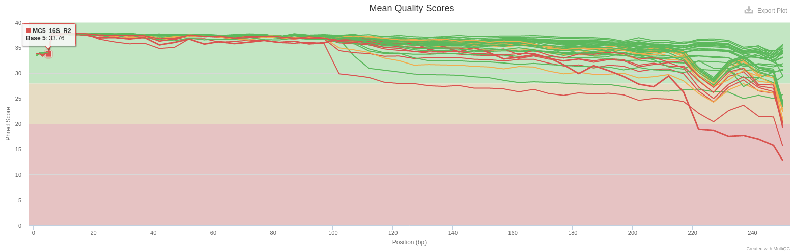
- Sequence Quality Histograms
- Mean quality scores are pretty good. Curve decreases a little more for MC5_R2. But the overlap of R1 and R2 can overcome that.
- All reads are 250 bases long. It indicates that no trimming has been previously performed
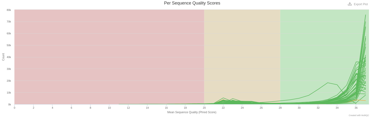
- Per Sequence Quality Scores
- The large majority of reads have a mean quality > 30 (99.9 % of confidence)
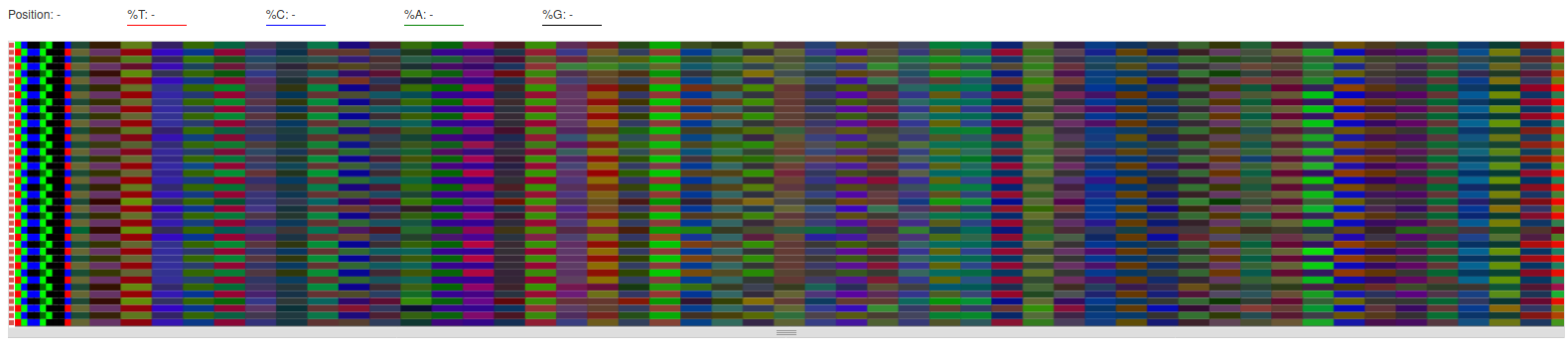
- Per Base Sequence Content
- We can see similar colors for R1 files and for R2 files at the beginning of the reads. They represent the primers.
- Per Sequence GC Content
- Not informative for amplicon data
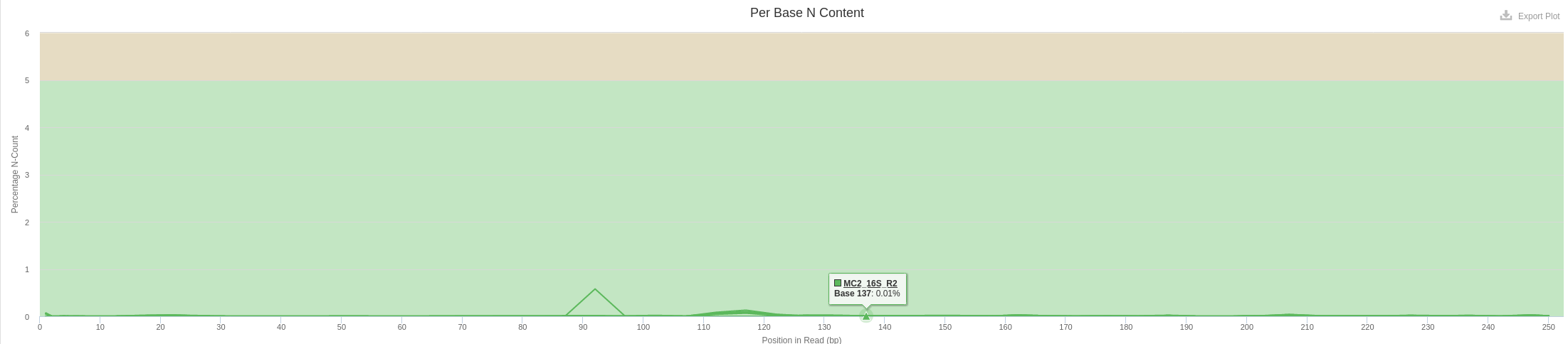
- Per Base N Content
- A small fraction of N bases are still present
- Sequence Length Distribution
- All reads are about 250 bases in size
- Sequence Duplication Levels
- Not informative for amplicon data
- Overrepresented sequences
- Not informative for amplicon data
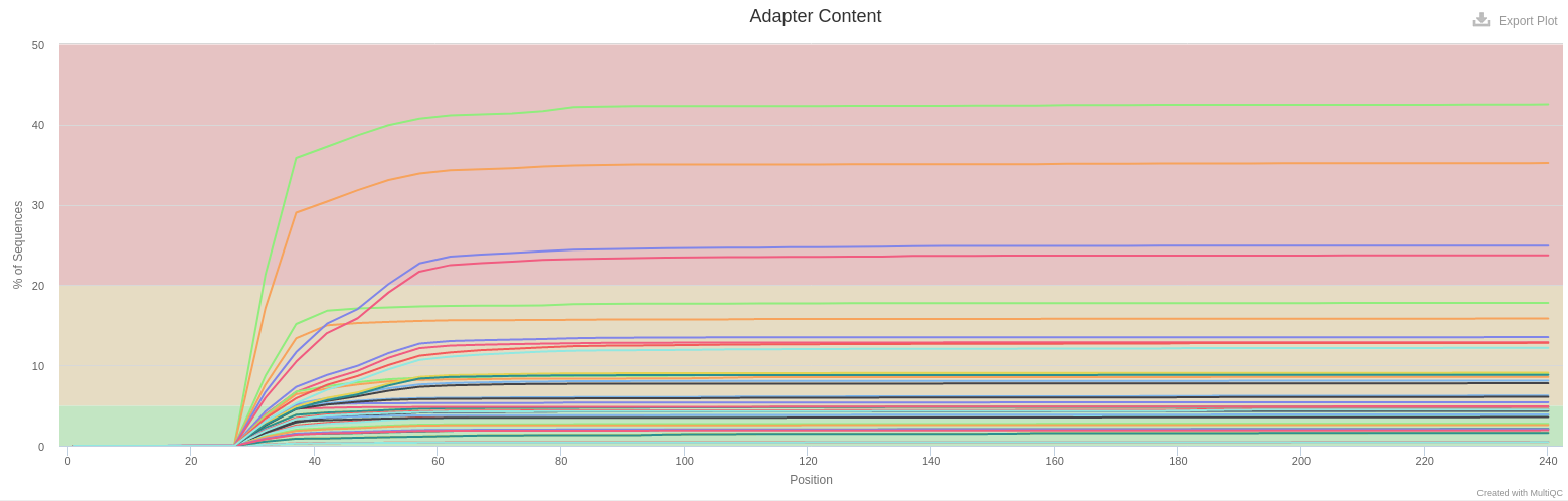
- Adapter Content
- Illumina adapters are present at different levels for all samples. It is representative of small fragments that have been sequenced. Those sequences will be removed later with FROGS.
FROGS
A good practice is to create an archive containing all FASTQ files. It is easier to manipulate than the 40 individual files.
tar zcvf data.tar.gz *.fastq.gzNow FASTQ files can be deleted because they are stored in the archive.
rm -f *.fastq.gz
# To extract files:
# tar xzvf data.tar.gz
Reads preprocessing
The knowledge of your data is essential. You have to answer the following questions to choose the parameters:
- Sequencing technology?
- Targeted region and the expected amplicon length?
- Have reads already been merged?
- Have primers already been deleted?
- What are the primers sequences?
Here are the answers for this dataset:
Sequencing technology
Type of data
Amplicon expected length
Primers sequences
Reads size
- 250 bp as seen previously
During the preprocess, paired-end reads are merged, filtered on length (according to min and max) and removed if they contain ambigous bases. Finally sequences are dereplicated to keep only one copy of each sequence. Counts per sample of each unique sequence are stored in the count matrix.
mkdir FROGS
qsub -cwd -V -N preprocess -o LOGS -e LOGS -pe thread 8 -R y -b y "conda activate frogs-4.1.0 && preprocess.py illumina --input-archive data.tar.gz --min-amplicon-size 200 --max-amplicon-size 490 --merge-software pear --five-prim-primer ACGGRAGGCWGCAGT --three-prim-primer AGGATTAGATACCCTGGTA --R1-size 250 --R2-size 250 --nb-cpus 8 --output-dereplicated FROGS/preprocess.fasta --output-count FROGS/preprocess.tsv --summary FROGS/preprocess.html --log-file FROGS/preprocess.log && conda deactivate"
Let look at the HTML file produced by FROGS preprocess to check what happened.
- 89.48% of raw reads are kept
- No overlap was found for ~8% of reads.
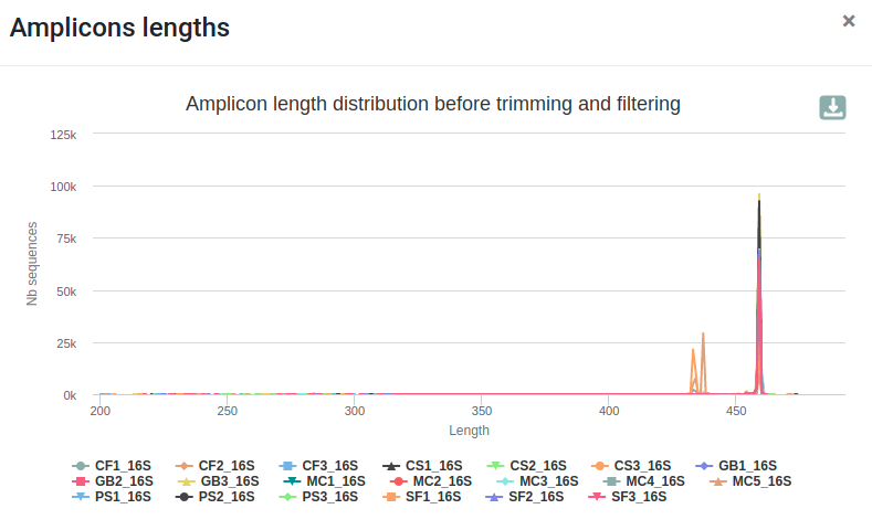
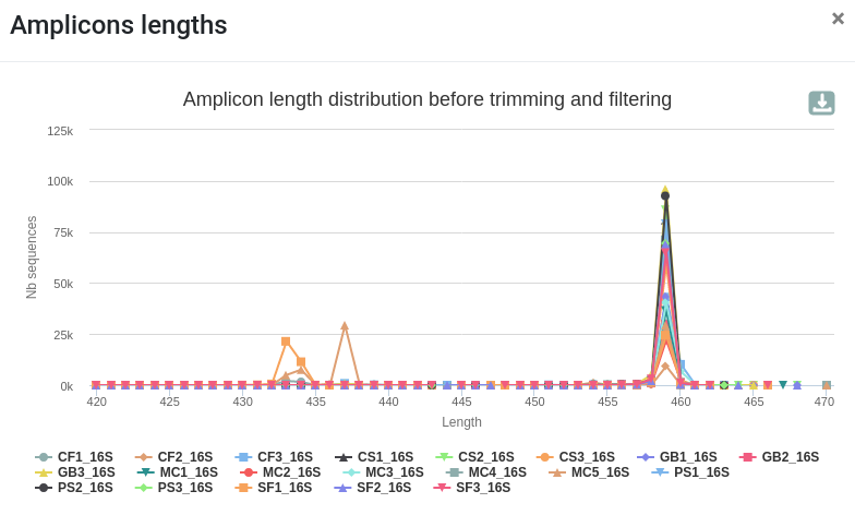
- The length distribution of sequences show that some sequences do not have the expected size.
- We can run this tool again to increase min amplicon size and reduce max amplicon size.
qsub -cwd -V -N preprocess -o LOGS -e LOGS -pe thread 8 -R y -b y "conda activate frogs-4.1.0 && preprocess.py illumina --input-archive data.tar.gz --min-amplicon-size 420 --max-amplicon-size 470 --merge-software pear --five-prim-primer ACGGRAGGCWGCAGT --three-prim-primer AGGATTAGATACCCTGGTA --R1-size 250 --R2-size 250 --nb-cpus 8 --output-dereplicated FROGS/preprocess.fasta --output-count FROGS/preprocess.tsv --summary FROGS/preprocess.html --log-file FROGS/preprocess.log && conda deactivate"Differences can be seen in the second HTML report.
Reads clustering
Following FROGS guidelines, swarm [6] is used with d=1 and --fastidious option.
qsub -cwd -V -N clustering -o LOGS -e LOGS -pe thread 8 -R y -b y "conda activate frogs-4.1.0 && clustering.py --input-fasta FROGS/preprocess.fasta --input-count FROGS/preprocess.tsv --distance 1 --fastidious --nb-cpus 8 --log-file FROGS/clustering.log --output-biom FROGS/clustering.biom --output-fasta FROGS/clustering.fasta --output-compo FROGS/clustering_compositions.tsv && conda deactivate"
qsub -cwd -V -N clusters_stats -o LOGS -e LOGS -b y "conda activate frogs-4.1.0 && cluster_stats.py --input-biom FROGS/clustering.biom --output-file FROGS/clusters_stats.html --log-file FROGS/clusters_stats.log && conda deactivate"
This report shows classical characteristics of clusters built with swarm:
- A lot of clusters: 122,281
- ~88% of them are composed of only 1 sequence
Chimera removal
The chimera detection is performed with vsearch [7].
qsub -cwd -V -N chimera -o LOGS -e LOGS -pe thread 8 -R y -b y "conda activate frogs-4.1.0 && remove_chimera.py --input-fasta FROGS/clustering.fasta --input-biom FROGS/clustering.biom --non-chimera FROGS/remove_chimera.fasta --nb-cpus 8 --log-file FROGS/remove_chimera.log --out-abundance FROGS/remove_chimera.biom --summary FROGS/remove_chimera.html && conda deactivate"This report shows classical results for chimera detection in 16S data:
- ~10% of sequences (20% of clusters) are chimeric
- Chimeric ckusters are made of few sequences
Abundance and prevalence-based filters
We now apply filters to remove low-abundant clusters that are likely to be chimeras or artifacts. We check also if some phiX sequences are still present. Low-abundant clusters are difficult to estimate. Following FROGS guidelines, we choose 0.005% of overall abundance. More stringent filters, including filters based on the prevalence across samples, can be made later if needed.
qsub -cwd -V -N filters -o LOGS -e LOGS -pe thread 8 -R y -b y "conda activate frogs-4.1.0 && cluster_filters.py --input-fasta FROGS/remove_chimera.fasta --input-biom FROGS/remove_chimera.biom --output-fasta FROGS/filters.fasta --nb-cpus 8 --log-file FROGS/filters.log --output-biom FROGS/filters.biom --summary FROGS/filters.html --excluded FROGS/filters_excluded.tsv --contaminant /db/outils/FROGS/contaminants/phi.fa --min-sample-presence 1 --min-abundance 0.00005 && conda deactivate"This report allows to show the impact of our filters:
- 180,483 clusters are filtered out; 195 clusters are kept!
- ~16% of sequences are lost but they mostly correspond to low-abundances clusters!
Affiliation
It is now time to give our clusters a taxonomic affiliation. We use the most up-to-date available version of Silva [8] (v.138.1) among all databanks available in the dedicated repository: /db/outils/FROGS/assignation/.
qsub -cwd -V -N affiliation -o LOGS -e LOGS -pe thread 8 -R y -b y "conda activate frogs-4.1.0 && taxonomic_affiliation.py --input-fasta FROGS/filters.fasta --input-biom FROGS/filters.biom --nb-cpus 8 --log-file FROGS/affiliation.log --output-biom FROGS/affiliation.biom --summary FROGS/affiliation.html --reference /db/outils/FROGS/assignation/silva_138.1_16S_pintail100/silva_138.1_16S_pintail100.fasta && conda deactivate"This report shows that all clusters were affiliated.
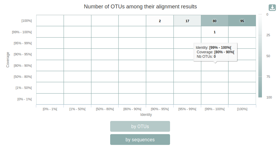
qsub -cwd -V -N affiliations_stats -o LOGS -e LOGS -b y "conda activate frogs-4.1.0 && affiliation_stats.py --input-biom FROGS/affiliation.biom --output-file FROGS/affiliations_stats.html --log-file FROGS/affiliations_stats.log --multiple-tag blast_affiliations --tax-consensus-tag blast_taxonomy --identity-tag perc_identity --coverage-tag perc_query_coverage && conda deactivate"You can use the Krona output to explore the affiliation.
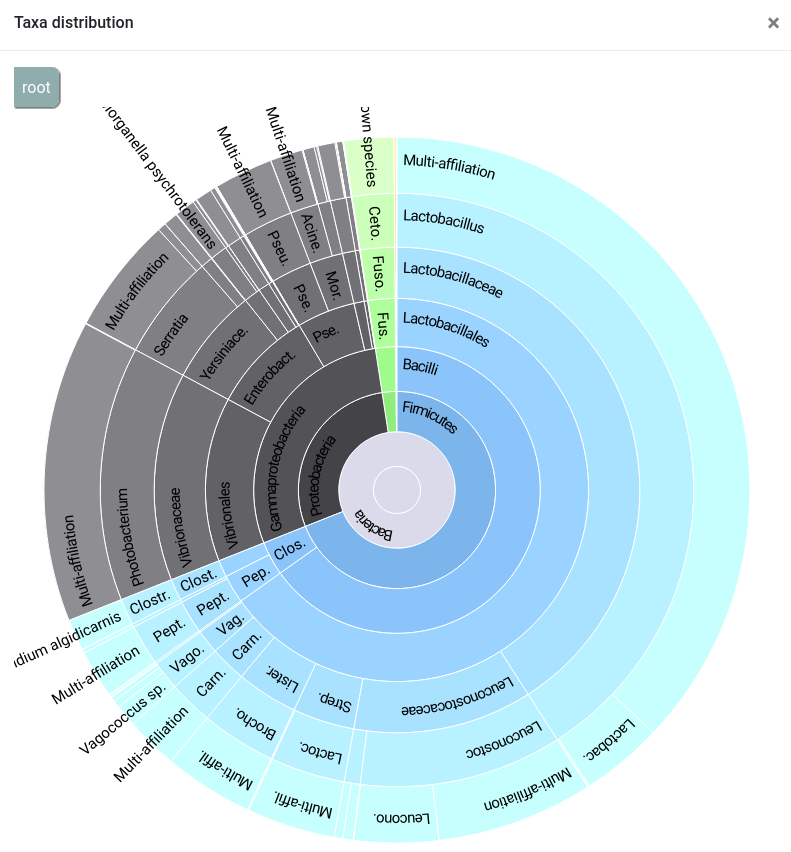
This report shows complementary informations about how clusters were affiliated. We can see that the 175 clusters have a blast coverage of 100% and a blast percentage identity > 99%. It can give you indications on supplementary filters to perform (remove clusters with too low coverage…).
qsub -cwd -V -N biom_to_tsv -o LOGS -e LOGS -b y "conda activate frogs-4.1.0 && biom_to_tsv.py --input-biom FROGS/affiliation.biom --input-fasta FROGS/filters.fasta --output-tsv FROGS/affiliation.tsv --output-multi-affi FROGS/multi_aff.tsv --log-file FROGS/biom_to_tsv.log && conda deactivate"Here are the results for our clusters, quite a few of them are multi-affiliated:
Multi-affiliations
FROGS uses blast tool against a reference databank to assign clusters. Particularly with 16S amplicon data, different species can harbor a similar, or even identical, 16S sequence in the targeted region. This is a very common phenomenon which explains why 16S analyses often do not discriminate between species within the same Genus. FROGS gives you the ability to view the conflicting affiliations of a given cluster. These are called multi-affiliations. Here is an example of a multi-affiliation:
| observation_name | blast_taxonomy | blast_subject | blast_perc_identity | blast_perc_query_coverage | blast_evalue | blast_aln_length |
|---|---|---|---|---|---|---|
| Cluster_4 | Bacteria;Firmicutes;Bacilli;Lactobacillales;Lactobacillaceae;Lactobacillus;Lactobacillus sakei | JX275803.1.1516 | 100.0 | 100.0 | 0.0 | 425 |
| Cluster_4 | Bacteria;Firmicutes;Bacilli;Lactobacillales;Lactobacillaceae;Lactobacillus;Lactobacillus curvatus | KT351722.1.1500 | 100.0 | 100.0 | 0.0 | 425 |
Sometimes it is useful to modify a multi-affiliation:
| observation_name | blast_taxonomy | blast_subject | blast_perc_identity | blast_perc_query_coverage | blast_evalue | blast_aln_length |
|---|---|---|---|---|---|---|
| Cluster_2 | Bacteria;Proteobacteria;Gammaproteobacteria;Vibrionales;Vibrionaceae;Photobacterium;unknown species | FJ456537.1.1524 | 100.0 | 100.0 | 0.0 | 425 |
| Cluster_2 | Bacteria;Proteobacteria;Gammaproteobacteria;Vibrionales;Vibrionaceae;Photobacterium;unknown species | FJ456356.1.1570 | 100.0 | 100.0 | 0.0 | 425 |
| Cluster_2 | Bacteria;Proteobacteria;Gammaproteobacteria;Vibrionales;Vibrionaceae;Photobacterium;Photobacterium phosphoreum | AB681911.1.1470 | 100.0 | 100.0 | 0.0 | 425 |
| Cluster_2 | Bacteria;Proteobacteria;Gammaproteobacteria;Vibrionales;Vibrionaceae;Photobacterium;Photobacterium phosphoreum | AY341437.1.1467 | 100.0 | 100.0 | 0.0 | 425 |
| Cluster_2 | Bacteria;Proteobacteria;Gammaproteobacteria;Vibrionales;Vibrionaceae;Photobacterium;Photobacterium phosphoreum | X74687.1.1457 | 100.0 | 100.0 | 0.0 | 425 |
You can use a dedicated Shiny application to do this easily through a nice interface: https://shiny.migale.inrae.fr/app/affiliationexplorer
Here is a video example illustrating the use of the app on our dataset:
Analysis of clusters
Phyloseq [3] is a R package dedicated to diversity analyses. It must be loaded in your R session prior to any analysis. You can do so using the following commands on the Migale Rstudio server: https://rstudio.migale.inrae.fr/.
Make a phyloseq object
To create a phyloseq object, we need the BIOM file, the metadata file and eventually a tree file (not generated here).
Go to your work directory:
library(phyloseq)
library(phyloseq.extended)
setwd("~/work/FROGS_16S")
biomfile <- "FROGS/affiliation.biom"
frogs <- import_frogs(biomfile, taxMethod = "blast")
metadata <- read.table("metadata2.txt", row.names = 1, header = TRUE, sep = "\t", stringsAsFactors = FALSE)
sample_data(frogs) <- metadata
frogs
phyloseq-class experiment-level object
otu_table() OTU Table: [ 195 taxa and 20 samples ]
sample_data() Sample Data: [ 20 samples by 7 sample variables ]
tax_table() Taxonomy Table: [ 195 taxa by 7 taxonomic ranks ]Here are the number of sequences before (red) and after (blue) the bioinformatics analyses, without additional curation or normalization.
samples <- rownames(sample_data(frogs))
final <- sample_sums(frogs)
initial <- metadata$Reads
final <- as.vector(t(final))
df <- data.frame(initial,final,samples)
df <- melt(df, id.vars='samples')
ggplot(df, aes(x=samples, y=value, fill=variable)) +
       geom_bar(stat='identity', position='dodge') +
      theme(axis.text.x = element_text(angle = 90, vjust = 0.5, hjust=1))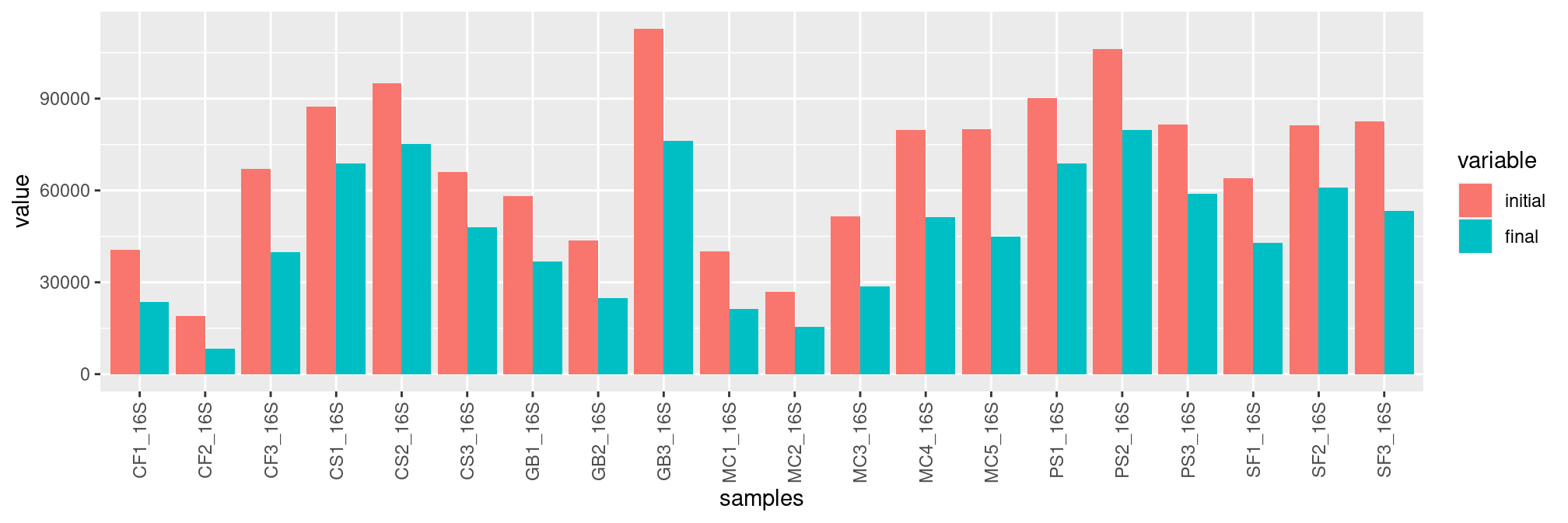
Phyloseq functions
From this object, you can apply a lot of functions to explore it. The full documentation is available here.
We can plot the composition of our samples at Phylum level with the function plot_bar(), ordered by EnvType metadata:
plot_bar(frogs, fill="Phylum") + facet_wrap(~EnvType, scales= "free_x", nrow=1)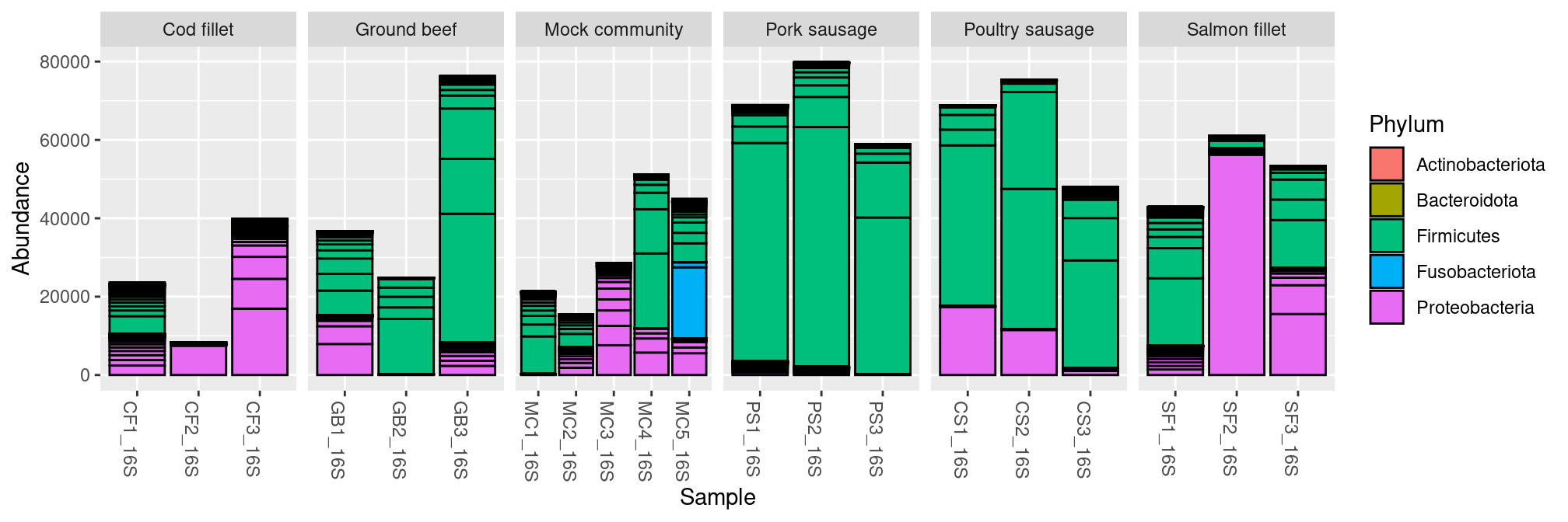
plot_composition() function allows to plot relative abundances:
plot_composition(frogs, taxaRank1 = NULL, taxaSet1 = NULL, taxaRank2 = "Phylum", numberOfTaxa = 10) +
  scale_fill_brewer(palette = "Paired") +
  facet_grid(~EnvType, scales = "free_x", space = "free_x")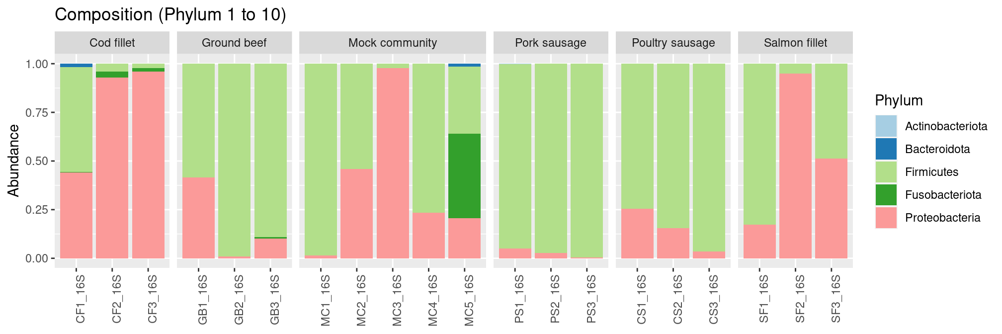
We can rarefy samples to get equal depths for all samples before computing diversity indices with function rarefy_even_depth().
frogs_rare <- rarefy_even_depth(frogs, rngseed = 20200831)Be careful with rarefaction, in this case a lot of sequences are lost because the smallest sample has so few sequences. Always check sample depths before rarefaction! You can remove poorly sequenced samples.
samples <- rownames(sample_data(frogs_rare))
non_rarefied <- sample_sums(frogs)
rarefied <- sample_sums(frogs_rare)
initial <- metadata$Reads
df <- data.frame(initial,non_rarefied,rarefied,samples)
df <- melt(df, id.vars='samples')
p <- ggplot(df, aes(x=samples, y=value, fill=variable)) +
      geom_bar(stat='identity', position='dodge') +
      ylab("sequences")+
      theme(axis.text.x = element_text(angle = 90, vjust = 0.5, hjust=1))
p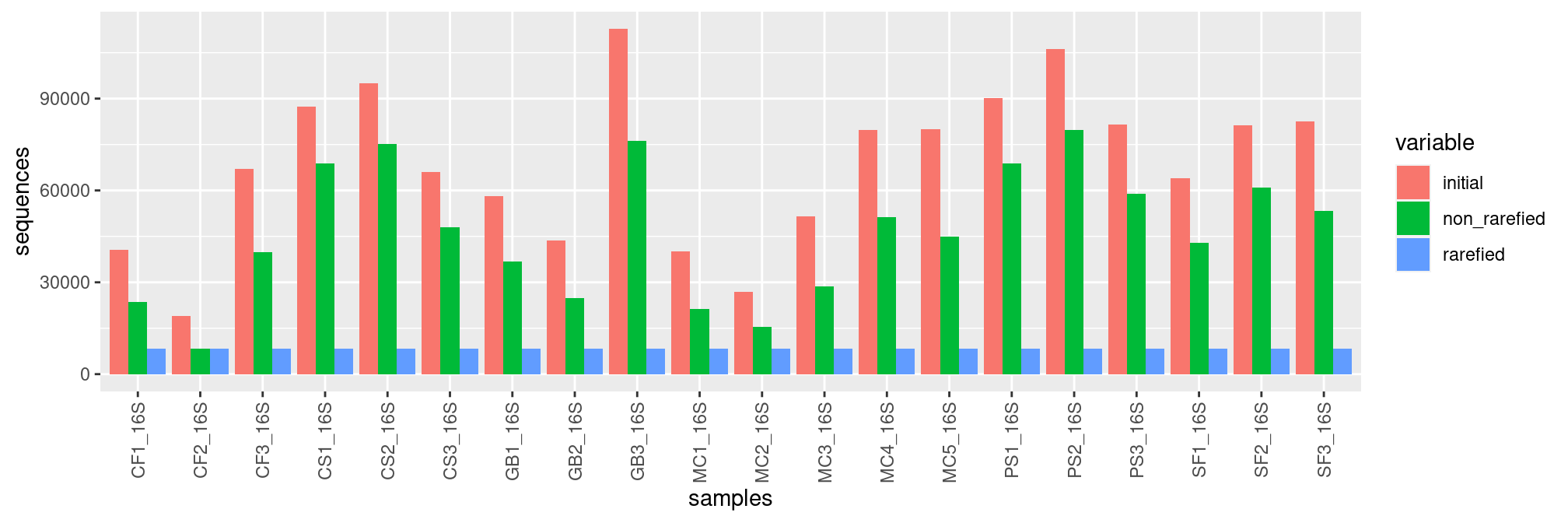
The rarefaction curves allow to see it too:
p <- ggrare(physeq = frogs, step = 100, se = FALSE, plot = FALSE) +
      ggtitle("Rarefaction curves") +
  aes(color = factor(EnvType)) +
  facet_wrap(~EnvType, scales = "free_y")
rarefying sample CF1_16S
rarefying sample CF2_16S
rarefying sample CF3_16S
rarefying sample CS1_16S
rarefying sample CS2_16S
rarefying sample CS3_16S
rarefying sample GB1_16S
rarefying sample GB2_16S
rarefying sample GB3_16S
rarefying sample MC1_16S
rarefying sample MC2_16S
rarefying sample MC3_16S
rarefying sample MC4_16S
rarefying sample MC5_16S
rarefying sample PS1_16S
rarefying sample PS2_16S
rarefying sample PS3_16S
rarefying sample SF1_16S
rarefying sample SF2_16S
rarefying sample SF3_16Sp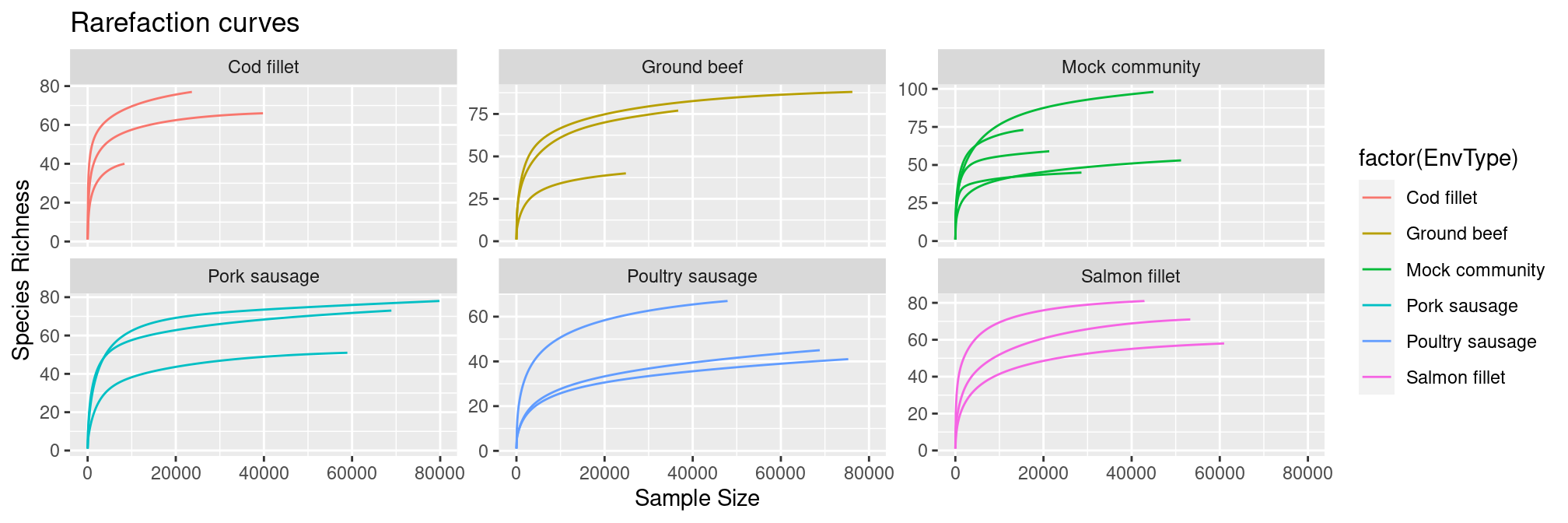
You can use a dedicated Shiny dedicated called easy16S to explore your phyloseq object easily and rapidly.
Here is a demonstration on this dataset:
The R commands used to generate the figures are available thanks to the button Show code. Once your figure is ready, you can copy the R instructions in your report for reproductibility and tweak it to adapt it to your needs.
A few conclusions
You have learned how to run FROGS on the migale server and to explore the results with easy16S. A small fraction of FROGS tools are presented here and some can be usefull for your own data (demultiplexing, phylogenetic tree, additional filters…). If you have any questions, you can contact us at help-migale@inrae.fr or at frogs-support@inrae.fr for FROGS specific questions.
References
1. Escudié F, Auer L, Bernard M, Mariadassou M, Cauquil L, Vidal K, et al. FROGS: Find, Rapidly, OTUs with Galaxy Solution. Bioinformatics. 2018;34:1287–94. doi:10.1093/bioinformatics/btx791.
2. Bernard M, Rué O, Mariadassou M, Pascal G. FROGS: a powerful tool to analyse the diversity of fungi with special management of internal transcribed spacers. Briefings in Bioinformatics. 2021;22. doi:10.1093/bib/bbab318.
3. McMurdie PJ, Holmes S. Phyloseq: An r package for reproducible interactive analysis and graphics of microbiome census data. PloS one. 2013;8:e61217.
4. Andrews S. FastQC a quality control tool for high throughput sequence data. http://www.bioinformatics.babraham.ac.uk/projects/fastqc/. 2010. http://www.bioinformatics.babraham.ac.uk/projects/fastqc/.
5. Ewels P, Magnusson M, Lundin S, Käller M. MultiQC: Summarize analysis results for multiple tools and samples in a single report. Bioinformatics. 2016;32:3047–8.
6. Mahé F, Rognes T, Quince C, Vargas C de, Dunthorn M. Swarm v2: Highly-scalable and high-resolution amplicon clustering. PeerJ. 2015;3:e1420.
7. Rognes T, Flouri T, Nichols B, Quince C, Mahé F. VSEARCH: A versatile open source tool for metagenomics. PeerJ. 2016;4:e2584.
8. Quast C, Pruesse E, Yilmaz P, Gerken J, Schweer T, Yarza P, et al. The SILVA ribosomal RNA gene database project: Improved data processing and web-based tools. Nucleic acids research. 2012;41:D590–6.

Sequencing quality is good. Nothing wrong detected at this step